This project is part of the CompuTop.org Software Archive.
Introducing Knoty
The goal of this Python Module is to provide an interactive framework for the visualization of Legendrian knots. It generates interactive 3D plots of Legendrian knots and contact structures. The final result is an interactive plot such as
Furthermore the module aims to provide a convenient way of reconstructing a 3D visualization from a front projection. The module can load in Bezier Curves from SVG files and plot the corresponding 3D structure. Consider the front projection
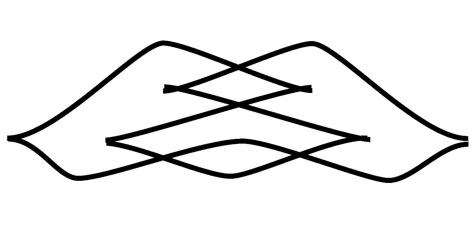
It was drawn in Inkscape using the Bezier Paths tool. Knoty can import the SVG file resulting in
Installation
The package can be installed from the Github repository via pip using
pip install git+http://github.com/slausmeister/knoty
The repository also includes a jupyter notebook illustrating the general workflow. All dependencies are installed automatically.
Dependencies
- K3D-Jupyter
- Numpy
- Sympy
- Matplotlib
- SvgPathTools
A note on K3D: K3D is a module that generates interactive 3D plots just like Matplotlib. In contrast to Matplotlib however K3D can utilize GPU acceleration. The difference is staggering.
Basic Usage
First we load the dependencies and the module
import knoty
import matplotlib.pyplot as plt
import numpy as np
import sympy as sp
The basic step of any visualization is to create a K3D plot, initialize objects on the plot and then visualize it. The visualizations are generated by functions provided in the knoty module. They always take in the plot and some arguments and return the plot with added information that is then plotted by k3d.display(). Therefore a cell always looks as follows:
plot = k3d.plot() # Create the K3D plot

plot = knoty.some_visualisation(plot, args) # Initialize some visualizations

plot.display() # Display the plot
Visualise Contact Structures
We can specify a Contact Form in Cartesian coordinates using the notation
form = [0, 'x', 1]
where the first entry describes the coefficient of the dx, the second entry the coefficient of dy and the third entry the coefficient of dz. We can also specify the three coordinates as coefficients using upticks. Therefore the expression above defines the form
\[xdy + dz\]i.e. the standard contact form. We can now plot the contact structure via the knoty.plot_contact_structure() function. The function needs the 3D plot as an input. An example is given by the following:
plot = k3d.plot()

form = [0, 'x', 1]
plot = knoty.plot_contact_structure(plot, form = form, alpha = 0.6)

plot.display()
The argument form specifies the form. If no form is given, then the function defaults to the standard contact form. The argument alpha sets the transparency of the contact planes and defaults to 0.5.
Visualise Legendrian Knots
There are two ways to specify Legendrian knots in knoty. Either trough an explicit equation or though a drawn front projection. For drawn front projections please see “Specifying knots through SVGs”.
To define a knot through an equation we first need to define a function for the knot as follows
def knot(t):
 return 3 * sp.sin(t) * sp.cos(t), sp.cos(t), sp.sin(t)**3
Make sure that the return contains three coordinates and that the components are defined in a Sympy compatible manner. Here for example we choose sp.sin instead of np.sin to get the sympy version of the sine function.
We can now plot the knot through the knoty.plot_knot() function. This function need the 3D plot and the function defining the knot. An example is given by the following:
plot = k3d.plot()

plot = knoty.plot_knot(plot, knot)

plot.display()
We can also plot contact planes along the knot through the knoty.plot_planes_along_knot() function. It again takes in the 3D plot and the knot equation. Additionally we can layer everything onto a single plot. For example, we could visualise the standard contact structure, plot the knot and indicate the contact planes in one 3D plot through the following code:
plot = k3d.plot()

plot = knoty.plot_contact_structure(plot)
plot = knoty.plot_knot(plot, knot)
plot = knoty.plot_planes_along_knot(plot, knot)

plot.display()
Specifying knots through SVGs
Knoty can import a front projection specified as an SVG using the knoty.import_from_svg() function. It returns a 3D Sympy equation that is compatible with the rest of the module. The path to the SVG needs to be specified as a string and given to the function as the first argument.
svg_file = './Examples/Blatt4A21.svg'  # Replace with your SVG file path

svg_knot = knoty.import_from_svg(svg_file) # Generate knot equation

# Proceed with any knoty function using svg_knot as the knot equation...
The import_from_knot() generates a plot of the imported front projection. This plot can be suppressed with the argument ‘show_front = False’.
Auto correction
To reduce the workload on the user, the import function attempts to correct the knot equation as to ensure continuity of the knot. The theory works as follows:
The x variable of the Legendrian knot is specified by
\[x = -\frac{dz}{dy}.\]Therefore for continuity, we need to ensure that all Bezier curves meet with the same derivative in the same (y, z) coordinate.
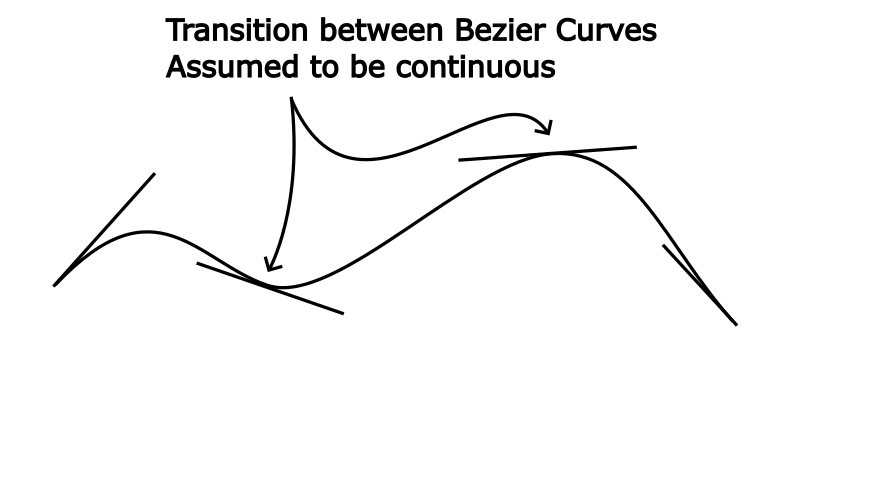
An SVG of Bezier Curves is organized in two layers. First we get a list of all continuous paths. Second each such list is a collection of linear or cubic Bezier curves specified by their control points. We assume that if a user draws a path in his/her vector graphics editor, that this path is already continuous.
Therefore we only worry about what happens, when the ends of two different paths come close to each other.
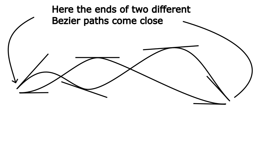
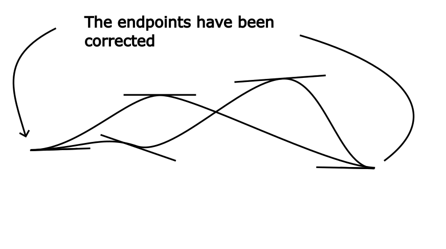
Here we assume, that the user is trying to draw a cusp. Therefore the function tries to auto correct the control points to achieve continuity. As discussed above, continuity is achieved if the curves meet tangentially. The simples way to achieve this is to first move the end points of the two different paths onto their average, ensuring (y, z) continuity and to then project their respective control points onto the horizontal going through that average point. Then, by the properties of Bezier curves, continuity is achieved.
During the import of the SVG the function will print out the corrections made
Correcting start point (0.15299824-7.6717687j)  and start point (0.17485513-7.6936256j)  to  (0.16392668500000002-7.68269715j)
Correcting end point (6.600781-6.6663516000000005j)  and start point (6.5789241-6.6007809j)  to  (6.58985255-6.63356625j)
To see if all necessary corrections were made, one might simply count the number of corrections and compare it to the number of cusps in the front.
The user can control this process using two arguments:
- threshold (float, default 0.1) sets the radius in which an end point searches for other end points. Modify this if not all cusps were recognized or if the auto correction wrongly groups path ends together
- correction (boolean, default True) sets whether the correction is performed. Useful if the front is crowded.
All in all this allows the user to draw a front without being too concerned about the exact Bezier curves. But be mindful of this feature, it may distort your knot. Notice how in the example the writhe of the knot changes.
Under github.com/slausmeister/knoty/tree/main/Examples you’ll find a few example SVGs as well as a template SVG. Keep in mind that the depth of the knot is directly proportional to the slope. Therefore steep slopes lead to a knot that explodes in depth.
Export to html
K3D plots can be exported to interactive html sites via the K3D control panel. The panel can be found in the plots under Controls/Snapshot HTML. The resulting html can either directly be accessed by a browser or can be integrated into another html via
<iframe src="/path/to/plot.html"></iframe>
Vignette
A short vignette can be found here or on the github.
TODO
- Full in code documentation
- Better scaling of SVG knots
- Export to sti for 3D printing
Acknowledgements
- Marc Kegel for holding an excellent lecture on Contact Geometry.
- Lenny Ng for providing me with the equations for his beautiful Legendrian knots from his Legendrian knot gallery.
- HEGL for technical support and all the 3D prints they have done.