<?xml version="1.0" encoding="utf-8"?><feed xmlns="http://www.w3.org/2005/Atom" ><generator uri="https://jekyllrb.com/" version="4.3.4">Jekyll</generator><link href="https://stani-stein.com//feed.xml" rel="self" type="application/atom+xml" /><link href="https://stani-stein.com//" rel="alternate" type="text/html" /><updated>2026-03-05T11:57:43+01:00</updated><id>https://stani-stein.com//feed.xml</id><title type="html">Stanislaus Stein</title><subtitle>Portfolio</subtitle><author><name>Stanislaus Stein</name><email>stanislaussteinvk@gmail.com</email></author><entry><title type="html">The Genodesic</title><link href="https://stani-stein.com//Genodesic/" rel="alternate" type="text/html" title="The Genodesic" /><published>2025-04-08T00:00:00+02:00</published><updated>2025-04-08T00:00:00+02:00</updated><id>https://stani-stein.com//Genodesic</id><content type="html" xml:base="https://stani-stein.com//Genodesic/"><![CDATA[<p>In Biology we’re often confronted with static snapshots of dynamic systems. A key task is to reconstruct the underlying dynamics from this snapshot. A prime example of such a task is trajectory reconstruction, where we try to find the typical path a cell takes whilst undergoing some process.</p>

<p>If we now assume that the system we’re observing is ergodic, then a sufficiently large sample size will contain all intermediate stages of the process. Hence the trajectory reconstruction becomes essentially a regression task on the dataset.
<img src="/assets/genodesic/spline_scatter_plot.png" alt="Scatter" /></p>

<p>Fig 1: We measure multiple cells, which all undergo the same dynamical process. Finding the typical development path boils down to computing a regression.</p>

<p>Finding such a regression path seems easy at first glance. But in the high dimensional data spaces commonly found in bioinformatics, the curse of dimensionality may quickly strike. Specifically the Euclidean metric can break down with an increase in dimensionality (see [Beyer et al.]). This is the detriment of most regression algorithms, such as principle curves, who often minimize some kind of Euclidean metric to the data. In the following we will not necessarily try to replace the Euclidean distances. Instead we want to enhance it with additional information to make it more robust in higher dimensions.</p>

<p>This blog post is concerned with the big picture concept of my master’s thesis and will delve a bit into how I simplified the modeling paradigm of an Information Geometry based regression algorithm, as well as into some technical aspects around the smoothness and stability of score estimates in the Hyvärinen sense. We will apply these techniques to single cell sequencing count data of cells undergoing stem cell reprogramming.</p>

<h1 id="mixing-in-some-information-geometry">Mixing in some Information Geometry</h1>

<p>[Sorrenson et al.] introduces the idea of constructing Geodesics with respect to a Fermat metric. In less mathematical terms this means the following: In Riemannian Geometry we allow our metric to vary as a function of the current position. One such choice for a metric is given by the Fermat metric, which rescales the normal Euclidean metric according to some property. In our case we rescale the Euclidean metric with respect to the density of the dataset at that point in such a way, that distances in high density regions become shorter, whilst distances in low density regions are enlarged. As our metric is derived from data, we’re firmly in the Information Geometry world. Our metric is given by</p>

\[g(u,v) := \frac{\langle u,v \rangle}{p^\beta},\]

<p>where $\langle u,v \rangle$ is the usual Euclidean metric, $p$ the density at the current position and $\beta$ some hyperparameter.</p>

<p>A Geodesic is now a curve, that (under appropriate assumptions) minimizes the length traveled between two points. In our case this means, that a curve going through the data will be shorter than a curve taking shortcuts through low density regions, as the distances are shorter where the data is. This has the effect, that solving a goedesic with respect to a Fermat metric will generate a curve, that will try to stick to the data.</p>

<p>In more mathematical terms, a geodesic $\gamma:[0,1] \to M$ minimizes the Length functional</p>

\[L(\gamma) := \int_0^1 \sqrt{g_{\gamma(t)}(\dot{\gamma}(t),\dot{\gamma}(t))} dt,\]

<p>where $g$ is the Fermat metric as defined above and $u$ and $v$ are tangent vectors at $\gamma(t)$. For length minimization we need to ensure that we use the correct Levi-Civita connection for our Geodesic equation $\nabla_\dot{\gamma} \dot{\gamma} = 0$. At the end we need to solve the following PDE (more details in [Sorrenson et al.])</p>

\[\ddot{\gamma} - 2\beta (s(\gamma) \cdot \dot{\gamma}) \dot{\gamma} + \beta s(\gamma) ||\dot{\gamma}||^2 = 0,\]

<p>where $s = \frac{\partial \log p}{\partial x}$ is the score in the sense of Hyvärinen and $\vert\vert \cdot \vert\vert$ the Euclidean norm. This PDE may be solved via a relaxation scheme, where we need to provide the start and endpoint we want to connect geodesically. We may also reframe it into an IVP, allowing us to predict the movement of a cell without a known endpoint. In this case however we also need to provide an initial direction of movement. Critically though in both cases we need access to the score of a position in the dataspace. We will return to this in just a second.</p>

<p><img src="/assets/genodesic/morph.gif" alt="Morph" /></p>

<p>Fig 2: Our relaxation of the Geodesic equation in action. We start with some initial path proposal connecting our desired start and end point. We update the curve using the score of the dataset.</p>

<h1 id="about-the-initialization">About the Initialization</h1>
<p>If we want to solve the PDE via relaxation, we need to provide it with an initial solution that will be iteratively refined. An initial guess might be given by the straight line connecting the start and end point. This proposal however is usually so far off the actual solution, that the relaxation scheme will fail to converge. Hence we need to come up with a smarter initial guess. [Sorrenson et al.] suggests to find an initial proposal using graph based methods. Specifically we construct a k-nearest neighbour (knn) graph with respect to the Euclidean norm. We then update the weights of the edges in the graph based on the density between the two nodes of the edge. A path proposal is now given by Dijkstra, which finds the shortest path between two points in the density based graph. The idea for the update of the edge weights is that locally the geodesic between two datapoints is given by a straight line in the Euclidean sense. The edge weight is approximated using</p>

\[dist(x_1, x_2) = \sum_{i = 1}^s \frac{|| y_i - y_{i-1}||}{p\big( y_{i - \frac{1}{2}} \big)},\]

<p>where $y_i$ are linear interpolates such that $y_0= x_1$ and $y_s = x_2$. Notice how we need to directly estimate the density of a point here instead of just the score.</p>

<h1 id="the-problem-with-the-scores">The Problem with the Scores</h1>
<p>[Sorrenson et al.] proposes to estimate the data via some normalizing flow (RQ-NSF [Durkan et al.]). This yields density estimates and in principle also the score via Autodiff. They noticed however, that calculating the score this way tends to produce rather noisy estimates. Hence, they resort to learning the score separately via sliced score matching to get around the AD stability issues. This separates our likelihood modeling from our score modeling. I wanted to investigate whether we can get around this issue by deriving the likelihood from a score model, rather than deriving the score estimate from a likelihood model.</p>

<p>The relevant comparisons are not quite straight forward. I’ve tested many different classical normalizing flow frameworks and whilst RQ-NSF is the most successful approach, it still is not convincing (see figure 7). Only when moving to a continuous normalizing flow framework do the results become acceptable. A relevant point of comparison is CellFlow by [Palma et al.], where they model sequencing count data using OT-CFM [Tong et al.]. This model can generate likelihoods by accounting for the divergence of the NeuralODE, as well as score estimates by employing an adjoint solver. It is thus a successful model, where the score is derived from the likelihood.</p>

<p>For my approach I choose to employ the VP-SDE from [Song et al.]. Unsurprisingly the generative capabilities of this approach are generally better then OT-CFM or RQ-NSF (see figure 7). We can also sample the network at $t=0$ to get a score estimate of the distribution. This is both in theory and in practice equivalent to DSM. Furthermore by considering the associated probability flow ODE ([Song et al.] appendix D), a VP-SDE set up can also provide likelihood estimates. Notice how the set up is mirrored in comparison to the original approach [Sorrenson et al.]. We directly model the score and derive a likelihood estimate from it. Thus we expect the scores to be somewhat better behaved. Another important side effect of this approach is, that generating a score via Autodiff, especially through an adjoint solver as found in the OT-CFM approach, is computationally speaking much more expensive than a simple neural net evaluation found in the VP-SDE approach.</p>

<p>We compare the score estimate on two benchmarks. By Taylor’s theorem we expect for a sufficiently regular function</p>

\[s(x + \epsilon) - s(x) = s'(x)\epsilon  + o(\epsilon^2),\]

<p>where $s’$ is the Jacobian of the score estimate. The key insight here is, that a stable score estimate should behave linearly under small perturbations until running into numerical issues. We hence compare $\vert\vert s(x + \epsilon) - s(x)\vert\vert $, where $\epsilon$ is just a deterministic perturbation vector. The results are shown in figure 3.</p>

<p><img src="/assets/genodesic/perturb.png" alt="Perturb" />
Fig 3: Comparison of the stability of the score estimates under small perturbations. We perturb the score at 12 random datapoints. The average is plotted in high opacity.</p>

<p>Notice how the VP-SDE approach both demonstrates a more linear behaviour, but also a lower variance between samples. For the OT-CFM approach the variance is at times so high, that it drops out of our logarithmic plot. Eventually both approaches run into numerical issues, but I’d argue that the VP-SDE approach is generally more stable and well behaved.</p>

<p>Another important property a good score estimate should have is a consistent direction under small perturbations. If the perturbation is small enough, then again by Taylor we have</p>

\[\begin{align*}
s(x)^\intercal s(x + \epsilon) &amp;= s(x)^\intercal (s(x) + s'(x) \epsilon + o(\epsilon^2))  \\
&amp;= s(x)^\intercal s(x) + s(x)^\intercal s'(x) \epsilon + o(\epsilon^2),
\end{align*}\]

<p>in words again a linear relationship. We again evaluate both models over multiple runs. The results are shown in figure 4.</p>

<p><img src="/assets/genodesic/angle.png" alt="Angle" />
Figure 4: Evaluating cosine similarities over perturbations. Again the variance may drop out of the log plot.</p>

<p>In this metric both approaches perform similarly. Interestingly enough we run into numerical instability faster then in the other benchmark. In our downstream application of the score estimate the VP-SDE approach also outperforms the OT-CFM approach, whilst requiring much less compute. These results aren’t necessarily surprising, as the adjoint solver used in the for the OT-CFM approach needs to not only solve an ODE, increasing compute, but also account for the divergence along the flow. Estimating this divergence with the Hutchinson trace estimator introduces Monte-Carlo effects. Thus the VP-SDE approach is generally to be preferred, as it not only provides smooth score estimates, increasing the stability of the geodesic relaxation, but also unifies score and likelihood modeling into a single framework.</p>

<h1 id="a-quick-demonstration-of-the-genodesic">A quick Demonstration of the Genodesic</h1>
<p>Going back to our application at hand we can solve the geodesic equation between two datapoints in the dataset. We use the VP-SDE model to both find the initial path proposal, as well as solving the geodesic equation via relaxation. This allows to perform a regression which is a bit more stable in higher dimensions, as we’re not relying as much on euclidean distances. An example of such a regression is shown in figure 5.</p>

<iframe src="/assets/genodesic/genodesic.html" style="width: 100%; height: 600px; border: none;"></iframe>
<p>Fig 5: A regression in the <a href="https://doi.org/10.1016/j.cell.2019.01.006">Schiebinger Dataset</a>. The initial proposal is in red, the relaxed curve in green. The coloring of the cells reflects the wallclock time provided by the dataset. The plot is a 3D UMAP of the 16 dimensional latent space. All computations are done in the latent space.</p>

<h1 id="evaluating-pseudotimes">Evaluating Pseudotimes</h1>

<p>The reason why we benchmark on the <a href="https://doi.org/10.1016/j.cell.2019.01.006">Schiebinger Dataset</a> is, that this dataset provides a wallclock time. Our Genodesic is also able to generate a pseudotime, as it is a parameterized curve. Even though the two times are not on the same scale, we can still compare their ordinality. We do this by considering the 10 nearest neighbours in the dataset of some points in our curve and averaging over them. This allows us to find the wallclock time in the immediate vicinity of the curve. We compare this estimate to our curve parameter. A good pseudotime estimate should be always rising in the wallclock time. If our wallclocktime decreases along our pseudotime, this would mean that our curve would go back in time and thus not capture the dynamics correctly.</p>

<p><img src="/assets/genodesic/pseudotime.png" alt="Pseudotime" /></p>

<p>Fig 6: Comparing the pseudotime to the wallclock time. A perfect estimate would be a diagonal line. Whilst the results aren’t great, they’re at least not terrible 🤷. The ordinality seems to be largely correct.</p>

<h1 id="generative-modeling-as-a-side-effect">Generative Modeling as a Side Effect</h1>
<p>All our approaches can not only provide density and score estimates, but can also perform generative modeling. We can use this as a sort of benchmark to get an impression about whether the model is actually capable of learning the underlying data. To benchmark this capability, we’re going to let all models generate exactly as many datapoints as there are in our training dataset. For each real datapoint we can then calculate the 10 nearest neighbours in both the real as well as the generated dataset. Dividing by 10 gives us a fraction for each datapoint, that indicates what the share of artificial datapoints around any real datapoint is. For a good model we’d expect this fraction to sit around 0.5, indicating an equal share of real and fake data. This provides a spatially-resolved view of model fit, unlike a single validation loss value, revealing which parts of the data manifold are well-captured or missed. We can also invert this analysis and consider the share of fake datapoints around each fake datapoint, indicating regions in the generated data, where the model invents stuff that is not backed by the data. The results of this analysis are shown in figure 7.</p>

<p><img src="/assets/genodesic/six.png" alt="Generative" />
Fig 7: Comparing generative capabilities. The top row shows the fraction of real datapoints around real datapoints. It thus answers “What did the model miss”. The bottom row shows the fraction of real datapoints around fake datapoints. It thus answers “What did the model invent”.</p>

<p>We can see in the top row of figure 7, that RQ-NSF is not capable of capturing the entire data manifold. There are significant regions, where there are essentially no datapoints around real datapoints. In contrast both OT-CFM as well as the VP-SDE seem to be largely alright on that front. In the bottom row we can see that both RQ-NSF as well as OT-CFM have parts, where there are only few real points around some generated points. Here the models are generating points in regions, that are not covered by the actual data. They are thus inventing data. Whilst these regions are also present in the VP-SDE model, I’d argue they’re less pronounced. This is actually really important for our genodesic, as a model that “fills in the blanks” will lead to a trajectory going through “invented biology”. Hence I conclude, that also on this front my VP-SDE approach outperforms the other models, as it not only beats the other models on all investigated benchmarks, but also makes the key improvement of combining the likelihood and score modeling needed into one unified model.</p>

<h1 id="minor-remarks">Minor Remarks</h1>
<p>Apart from the usual Bioinformatics workflow of filtering count datasets to find highly variant genes, we are also using an Autoencoder to reduce ~1500 highly variable genes to a 12 dimensional latent space. This Autoencoder replaces the standard PCA. Instead of a standard reconstruction loss however, it is better to explicitly consider the Negative Binomial (NB) distribution of count data. Whilst this methodology is a bit novel, I still didn’t find it appropriate to include it in the discussion above, as geodesic trajectory reconstruction works in general continuous dataspaces. Yet still, the NB-Autoencoder should merit a future blog entry.</p>

<h1 id="possible-improvements">Possible Improvements</h1>
<p>Currently most compute is spend on generating the initial path proposal. This is because we calculate a knn of the dataset and then update each edge using the density estimated provided by the probability flow ode. Thus we have to run a lot of network evaluations per edge for a lot of edges. We do this as a naive proposal such as a straight line usually goes through very sparse regions of the latent space. The scores in these regions are very uninformative, leading to a failure of convergence. Notice how this is one of the problems also encountered and solved in [Song et al.]. Here they noticed, that we can get more sensible score estimates for sparse regions by inflating the noise perturbation. As this is already the model we employ, we might construct a relaxation scheme, where we initialize with a straight line and gradually reduce the noise over time. Thus our early curve will still have informative scores, whilst later relaxation steps should be able to make use of more detailed score estimates. Thus we may be able to completely cut out the graph based parts of our pipeline, significantly reducing compute.</p>

<h1 id="references">References</h1>
<p>[Beyer et al.] Kevin Beyer, Jonathan Goldstein, Raghu Ramakrishnan, Uri Shaft “When Is “Nearest Neighbor” Meaningful?”</p>

<p>[Sorrenson et al.] Peter Sorrenson, Daniel Behrend-Uriarte, Christoph Schnörr, Ullrich Köthe “Learning Distances from Data with Normalizing Flows and Score Matching”</p>

<p>[Palma et al.] Alessandro Palma, Till Richter, Hanyi Zhang, Andrea Dittadi, Fabian J Theis “cellFlow: a generative flow-based model for single-cell count data”</p>

<p>[Song et al.] Yang Song, Jascha Sohl-Dickstein, Diederik P. Kingma, Abhishek Kumar, Stefano Ermon, Ben Poole “Score-Based Generative Modeling through Stochastic Differential Equations”</p>

<p>[Tong et al.] Alexander Tong, Kilian Fatras, Nikolay Malkin, Guillaume Huguet, Yanlei Zhang, Jarrid Rector-Brooks, Guy Wolf, Yoshua Bengio “Improving and generalizing flow-based generative models with minibatch optimal transport”</p>

<p>[Durkan et al.] Conor Durkan, Artur Bekasov, Iain Murray, George Papamakarios “Neural Spline Flows”</p>]]></content><author><name>Stanislaus Stein</name><email>stanislaussteinvk@gmail.com</email></author><summary type="html"><![CDATA[Trajectory Reconstruction using Geodesics with respect to a Distance Based Metric learned via Score Matching applied to sequencing count data.]]></summary></entry><entry><title type="html">When Massive Parallelism Is Not Enough: Optimizing the Hamming Matrix</title><link href="https://stani-stein.com//Hamming/" rel="alternate" type="text/html" title="When Massive Parallelism Is Not Enough: Optimizing the Hamming Matrix" /><published>2025-02-06T00:00:00+01:00</published><updated>2025-02-06T00:00:00+01:00</updated><id>https://stani-stein.com//Hamming</id><content type="html" xml:base="https://stani-stein.com//Hamming/"><![CDATA[<p>Topological Data Analysis (TDA) is concerned with finding topological invariants of a data set. This allows us to find circular relationships in datasets, as a circle can be seen as a hole in the data manifold and hence can be described by topology. This can for example be used to find beneficial mutations in viral evolution (see for example [Bleher et al.]).</p>

<p>To perform the TDA, we are given a point cloud dataset $X \subset \mathbb{R}^d$ with a metric $d(x,y)$, where $x, y \in X$. We now calculate the distance between each data point and summarize it in a distance matrix. We then generate the Vietoris–Rips complex from this Hamming matrix and compute the persistent homology of the dataset, which summarizes the topological invariants.</p>

<p>We can apply this approach to a collection of viral genomes. The natural metric here is the Hamming distance, which counts the number of positions where two genomes differ. Thus to compute an entry in the Hamming matrix we load in two sequences and compare them at each index with a simple XOR. Afterwards we sum along the XOR sequence to get the distance between the two sequences.</p>

<p><img src="/assets/Hamming/xor.png" alt="XOR" /></p>

<p>Notice how each comparison is independent of all the others and that computing an entry in the Hamming matrix is independent of all other entries. My initial naive thought was that using the right tensor operations in PyTorch, we could perform all these computations simultaneously and then simply sum up the results. This seemed like exactly what GPUs are built for. Boy was I wrong!</p>
<h1 id="the-naive-approach">The naive Approach</h1>
<p>The dataset can be viewed as a $n \times d$ matrix where $n$ refers to the number of genomes. We can create $n$ shallow copies of each sequence along a new index leading to the following tensor:
<img src="/assets/Hamming/tensor.png" alt="Tensor" />
Here the sequences go from front to back. Each unique sequence is given a unique color, every copy is assigned the same color. The new index goes from left to right, hence leading to horizontal stacking of the replicated data matrix.</p>

<p>We can now transpose this tensor and overlap it with itself to get the interaction of each sequence in the dataset with all the others. Afterwards we perform the XOR at every overlapping sequence creating a new 3D tensor. We now sum front to back to get the final Hamming matrix. This can be summarized in the following animation.</p>

<p><img src="/assets/Hamming/merge.gif" alt="Merge" /></p>

<p>The beauty of this approach is twofold: First, all comparisons happen in principle at the same time thus maximizing parallelization and second, it is very easy to implement in PyTorch:</p>

<div class="language-python highlighter-rouge"><div class="highlight"><pre class="highlight"><code><span class="n">n</span><span class="p">,</span> <span class="n">d</span> <span class="o">=</span> <span class="n">tensor_dna</span><span class="p">.</span><span class="nf">size</span><span class="p">()</span>
<span class="n">left</span> <span class="o">=</span> <span class="n">tensor_dna</span><span class="p">.</span><span class="nf">unsqueeze</span><span class="p">(</span><span class="mi">1</span><span class="p">).</span><span class="nf">expand</span><span class="p">(</span><span class="n">n</span><span class="p">,</span> <span class="n">n</span><span class="p">,</span> <span class="n">d</span><span class="p">)</span>
<span class="n">top</span> <span class="o">=</span> <span class="n">tensor_dna</span><span class="p">.</span><span class="nf">unsqueeze</span><span class="p">(</span><span class="mi">0</span><span class="p">)</span>
<span class="n">diff</span> <span class="o">=</span> <span class="n">left</span> <span class="o">!=</span> <span class="n">top</span>
<span class="n">hamming_matrix</span> <span class="o">=</span> <span class="n">diff</span><span class="p">.</span><span class="nf">sum</span><span class="p">(</span><span class="n">dim</span><span class="o">=</span><span class="mi">2</span><span class="p">)</span>
</code></pre></div></div>
<p>Whilst this makes for some very elegant code, it fails spectacularly in comparison to even the simplest CPU implementation. It took me a lecture on GPUs to find out why.</p>

<h1 id="the-very-basics-of-gpu-computing">The very Basics of GPU computing</h1>
<p>A modern Nvidia GPU basically consists of</p>
<ul>
  <li>Streaming Multiprocessors (SMs): Computing blocks with local memory that can process data from and into local memory and request new data from global memory</li>
  <li>Global Memory: A global memory resource, that can be accessed by all SMs</li>
  <li>A lot of infrastructure connecting everything</li>
</ul>

<p><img src="/assets/Hamming/Ada.png" alt="Ada" />
An overview of the architecture of an RTX 4090. Notice the abundance of SMs on the chip. Each SM has its own memory and L1 cache. The L2 cache is shared amongst all SMs on the die. Global memory is an off-chip resource and thus not shown. Also, the RTX 4090 is a gaming GPU and thus has a lot of functionality for computer graphics. It can be safely ignored for this discussion. (Source: Ada Lovelace Whitepaper)</p>

<p>Instead of executing functions on a GPU, CUDA instead launches a kernel. It is in many ways similar to a C++ function, but instead of executing one, it spawns many different threads executing the same function. To control this parallelism, we specify a block and a grid size.</p>

<p>The block size determines how many threads of the function we want to spawn on a single SM. Different threads execute the same instructions on different data. We can execute up to 1024 threads on a single SM. For the actual execution the GPU groups up to 32 threads into what is called a warp. A scheduler now chooses a warp for execution, which is then executed in a SIMD style. Thus we pretty much always execute 32 threads at the same time on a single SM. As all threads in a block reside on the same SM, they can communicate with each other. We need to keep in mind however that a priori it is not guaranteed, that all threads are at the same instruction of the kernel. To prevent threads from illegal memory accesses or working on stale data we need to synchronize them. For more on this see [Valiant].</p>

<p>If 1024 threads are not sufficient, we can use the grid size parameter. It determines on how many SMs the function will be executed. Consider for example a grid size of 20 with a block size of 512. The GPU will now execute the function on 20 SMs, each with 512 threads. The drawback here is that threads can not communicate or even be synchronized across different SMs. Thus, the only way for a thread on SM A to pass information to a thread on SM B is to write the result to global memory, terminate the kernel, and then relaunch it. This kernel relaunch is the only way to guarantee that all threads from a kernel are at the same instruction of the kernel.</p>

<p>One of the key tricks that GPUs use to achieve high performance is called parallel slackness. Unlike CPUs, GPUs can switch between different warps extremely quickly when a warp stalls, such as when waiting for data from global memory—a delay that can easily cost 100 clock cycles. Instead of idling during this wait, the GPU scheduler immediately switches execution to another warp that’s ready to run. This rapid context switching effectively hides memory latency and keeps GPU resources utilized. However, to fully benefit from parallel slackness, the GPU needs enough warps queued up and ready; otherwise, the SM stalls and performance suffers. GPUs use a similar strategy at the block level, but that’s beyond our scope here.</p>

<p><img src="/assets/Hamming/parallel_slackness.gif" alt="Context-Swtiching" />
Parallel slackness in action: The SM works on a warp until it stalls. It then switches to a warp that is ready for execution. Stalled warps should become ready for execution as soon as the high latency operation, such as a memory access, is completed. If no warp is ready for execution, the entire SM stalls.</p>

<h1 id="the-culprit-of-the-hamming-matrix-arithmetic-intensity">The Culprit of the Hamming Matrix: Arithmetic intensity</h1>
<p>Arithmetic intensity measures how many operations are performed per byte loaded. We usually target a value of at least 100. This ensures that by the time new data needs to be loaded in, another warp has already completed its memory request. Our Hamming distance is in many ways the worst case. We can represent each base pair as a single byte. Per base pair we only need to perform a single XOR operation and a few additions, which are highly optimized on GPUs. Thus we are constantly stalling as we’re waiting for the next base pairs to be loaded in. I suspect that this is where the PyTorch implementation is failing.</p>

<p>Fortunately, CUDA allows us to parallelize not only execution but also memory transactions by bundling multiple data fetches into fewer memory operations. From a machine learning perspective we might say that we work in batches. This however takes an explicit effort on the part of the programmer. I found the most important optimization to be transposing one of the arrays on the CPU before copying both onto the GPU. This allows the memory controller to load in the data in a coalesced manner, if we carefully reason through what data needs to be loaded when. What is meant exactly by this is again beyond the scope of this post, but a good reference can be found in [Kirk et al.].</p>

<p>Nsight Compute, a profiler by Nvidia gives us some insight about the performance of our code. The most important for us is the estimate of the computational intensity. In contrast to the arithmetic intensity, which is concerned with the theoretical arithmetic, the computational intensity is concerned with the operations per byte of the actual performance. To understand our kernel Nsight Compute provides the roofline chart.</p>

<p><img src="/assets/Hamming/roofline.png" alt="Roofline" />
The roofline chart plots computational intensity against peak performance. There are two break-even points, one for fp32 and one for fp64. If we’re left of these break even points our kernel is memory bound. The maximum performance is then given by the solid blue line. Any improvements in computational speed are negated by warps stalling as they wait for new data. Kernels sitting to the right of the break-even point are referred to as compute bound. Here smarter computations do bring tangible performance benefits.</p>

<p>For the longest time I though that Nsight Compute was not properly profiling my kernel, as I did not find the marker indicating our performance in the roofline plot. It is however there, at the bottom left corner. Notice how it is actually below one as we’re performing some clever byte packing (and also unfortunately load in some redundant data).</p>

<p>Nevertheless, with careful memory management, GPUs can still significantly outperform CPUs in computing Hamming distances. I currently benchmark a 20 fold improvement against a SIMD based C++ implementation. We do however lose again to the CPU when it comes to very large data sets that no longer fit onto the global memory of the device. Here we’d have to stream in data from system memory over PCI express, which carries a much higher penalty than the already very high penalty of global memory accesses.</p>

<h1 id="final-verdict-and-a-note-on-future-developments">Final Verdict and a Note on Future Developments</h1>

<p>As we have seen, for good GPU performance we not only need to construct problems that can be broken down into independent sub problems, we also need a sufficiently high arithmetic intensity to not stall for memory requests. Fortunately, matrix multiplication—the backbone of modern machine learning—requires $2N^2$ loads and $2N^3$ operations when multiplying two square matrices. Thus our arithmetic intensity scales linearly in matrix size.</p>

<p>As stated I currently target an arithmetic intensity of at least 100. With future GPUs we do however expect both the compute as well as the memory sub system to improve. We can quickly estimate a good target for any GPU by dividing the peak Float32 performance by the Memory bandwidth. While simplified, this helps guide initial performance expectations and optimization efforts. For the 4090 this gives a target of ~80. Generally we however expect that compute improves faster than memory. Thus in the long run kernels need to be more compute heavy to fully utilize a GPU. Thus, neural networks will likely need to grow even larger to scale effectively with future increases in computational capability.</p>
<h1 id="references">References</h1>

<p>[Bleher et al.] Bleher, Michael et al. “Topology identifies emerging adaptive mutations in SARS-CoV-2” arXiv preprint arXiv:2106.07292 (2021)</p>

<p>[Valiant] Valiant, Leslie G. “A bridging model for parallel computation”</p>

<p>[Kirk et al. ] Kirk, David and Hwu, Wen-mei “Programming Massively Parallel Processors: A Hands-on Approach”</p>]]></content><author><name>Stanislaus Stein</name><email>stanislaussteinvk@gmail.com</email></author><summary type="html"><![CDATA[Computing the Hamming Matrix suits GPU parallelism, but its low arithmetic intensity demands careful memory optimization to beat CPUs.]]></summary></entry><entry><title type="html">Fixing Lightroom’s Automatic Photo Adjustment using Machine Learning</title><link href="https://stani-stein.com//AutoHDR/" rel="alternate" type="text/html" title="Fixing Lightroom’s Automatic Photo Adjustment using Machine Learning" /><published>2024-07-02T00:00:00+02:00</published><updated>2024-07-02T00:00:00+02:00</updated><id>https://stani-stein.com//AutoHDR</id><content type="html" xml:base="https://stani-stein.com//AutoHDR/"><![CDATA[<p>*joint work with <a href="https://lucas-schmitt.de">Lucas Schmitt</a>.</p>

<p>Note: By now Adobe has implemented proper HDR settings making the workflow below redundant.</p>

<p>Best viewed in an HDR compatible browser (Chrome) on an HDR compatible display.</p>

<h1 id="abstract">Abstract</h1>
<p>This project develops an algorithm to optimize high dynamic range (HDR) image editing settings in Adobe Lightroom for RAW images. Current auto-adjustment algorithms do not fully utilize HDR’s expanded brightness spectrum, resulting in less dynamic images. Our solution employs a Vision Transformer (ViT) model trained on a small dataset of RAW images with corresponding Lightroom settings. The model predicts optimal adjustments for exposure, contrast, highlights, shadows, whites, blacks, vibrance, and saturation, enhancing HDR image quality. Key techniques include data augmentation and label smoothing to improve model performance. This algorithm offers photographers a tool for achieving superior HDR image enhancements with minimal manual adjustments.</p>

<h1 id="introduction">Introduction</h1>
<p>Modern photography software like Adobe Lightroom and Darktable play a crucial role in the digital photography workflow, particularly for photographers who shoot in RAW format. RAW files contain unprocessed data directly from a camera’s image sensor, preserving the highest possible quality and providing extensive flexibility for post-processing. Unlike JPEGs, which are compressed and processed in-camera, RAW files allow photographers to make significant adjustments to exposure, color balance, contrast, and other parameters without degrading image quality. This capability is essential for professional photographers and enthusiasts seeking to achieve the highest quality results.</p>

<p>The workflow of shooting in RAW typically begins with capturing images using a camera set to save files in the RAW format. These files are then imported into software like Lightroom or Darktable, where photographers can adjust various settings to enhance the images. The software offers a wide range of tools for fine-tuning, such as adjusting white balance, exposure, shadows, highlights, and color saturation. This non-destructive editing process means that the original RAW file remains unchanged, and all adjustments are stored as metadata. This allows for endless experimentation and refinement until the desired outcome is achieved. The RAWs themself are usually captured as neutral as possible allowing the most flexibility in edit. This however also means that the RAWs are usually quite flat and grey, making the editing of every photo almost a necessity.</p>

<p>Given the complexity and variety of adjustments available, finding the optimal settings can be a time-consuming process, especially if one edits a large set of images of an event. Therefore most photographers are deeply familiar with Lightroom’s Auto Settings (Shift + A). This algorithm suggests values for some of the most important settings (Exposure, Contrast, Highlights, Shadows, Whites, Blacks, Vibrance, Saturation and some more). Most of the time these suggestions yield vibrant pictures that only need small adjustments to a subset of these settings. Therefore, a usual workflow might be to apply autosettings to all images and to only retouch a subset of the settings for each image, saving a lot of time.</p>

<h2 id="hdr-photography">HDR Photography</h2>
<p>Since October 2023 Adobe Lightroom has added native support for high dynamic range (HDR) image editing. HDR images contain more data per pixel, allowing the image to reach higher brightness values without oversaturating shadows. An HDR compatible display will now be able to ramp up the brightness of these areas significantly, whilst still keeping the shadows dark.</p>

<p>You can check if your current display supports HDR by comparing the images below. If they appear similar, then your display does not support HDR. On a proper HDR display the sun on the right picture should almost be blinding and shadows should be rich in detail, just as your eye would experience it in real life.</p>

<table>
  <tr>
    <th>Unedited Raw</th>
    <th>Non HDR Image</th>
    <th>HDR Image</th>
  </tr>
  <tr>
    <td><img src="/assets/AutoHDR/unedited.jpg" width="200" /></td>
    <td><img src="/assets/AutoHDR/non_hdr_expl.jpg" width="200" /></td>
    <td><img src="/assets/AutoHDR/hdr_expl.jpg" width="200" /></td>
  </tr>
</table>

<p>Fig 1: The image on the left is an unedited RAW image, the one in the middle has been edited and exported using a standard non HDR workflow and the image on the right with an HDR workflow. If the two edited images appear the same to you, then your browser/display do not support HDR playback.</p>

<p>HDR technology is still in its early stages, so most displays do not support it yet. However, your phone might, as it typically offers the best display quality for the average consumer. Most laptops can not increase the brightness of a subset of pixels significantly without also increasing the brightness of dark parts. Therefore the bright parts of the HDR image are artificially darkened, destroying the HDR effect.</p>

<p>The only problem with Adobe’s HDR implementation is that the autosettings do not consider the expanded brightness space. They tend to compress the brightness scale down to the usual allowed brightness scale. Therefore the blinding sunset becomes just bright and the dark shadow becomes brighter. The whole image now seems as grey as if it were not using HDR. A photographer would now need to adjust every single setting to restore the HDR effect, negating the usefulness of the autosettings.</p>

<table>
  <tr>
    <th>Adobe Autosettings</th>
    <th>Model Predicted Autosettings</th>
  </tr>
  <tr>
    <td><img src="/assets/AutoHDR/AdobeHDR.jpg" width="200" /></td>
    <td><img src="/assets/AutoHDR/AutoHDR.jpg" width="200" /></td>
  </tr>
</table>

<p>Fig 2: On the left the settings suggested by Lightroom, on the right the settings suggested by our algorithm. Notice how Lightroom’s implementation boosts the shadows and is not using the entire brightness spectrum available. We again point out the necessity for an HDR compatible browser/display.</p>

<p>The aim of the project is to write an algorithm that, given a small training dataset of RAWs with the corresponding Lightroom settings, finds a good suggestion for the settings to properly make use of the HDR colorspace.</p>

<h1 id="architectural-concerns">Architectural Concerns</h1>

<p>Our model has 8 settings to play with. <em>Exposure</em> adjusts overall brightness, ensuring a balanced level where both shadows and highlights retain detail without overexposure or underexposure. <em>Contrast</em> controls the difference between dark and light areas, essential for HDR. <em>Highlights</em> manage brightness in lighter parts, crucial for avoiding overexposure and maintaining detail in bright regions. <em>Shadows</em> adjust brightness in darker areas, vital for revealing details without making them unnaturally bright. Similarly one can adjust <em>Whites</em>, <em>Blacks</em>, <em>Vibrance</em> and <em>Shadows</em>. That is why our model needs to understand the effect of the settings on both the darkest and the brightest areas of the images at the same time. In other words, we have long range dependencies. Our choice therefore lands on the Vision Transformer introduced in [Dosovitskiy et al., 2020].</p>

<p>The settings are all in the interval (-100,100) except for Exposure which lies in (-5,5). So, we scale all these intervals down to (-1,1) and train our model to $(-1,1)^n$ by choosing $\operatorname{tanh}()$ as the final activation of our ViT. After training we rescale the logits to use them in Lightroom. To use the standard Google ViT, we replace the final layer as follows:</p>

<div class="language-python highlighter-rouge"><div class="highlight"><pre class="highlight"><code><span class="n">model</span> <span class="o">=</span> <span class="nc">ViTForImageClassification</span><span class="p">(</span><span class="n">config</span><span class="p">)</span>

<span class="n">model</span><span class="p">.</span><span class="n">classifier</span> <span class="o">=</span> <span class="n">nn</span><span class="p">.</span><span class="nc">Sequential</span><span class="p">(</span>
    <span class="n">nn</span><span class="p">.</span><span class="nc">Linear</span><span class="p">(</span><span class="n">model</span><span class="p">.</span><span class="n">config</span><span class="p">.</span><span class="n">hidden_size</span><span class="p">,</span> <span class="n">self</span><span class="p">.</span><span class="n">num_classes</span><span class="p">),</span>
    <span class="n">nn</span><span class="p">.</span><span class="nc">Tanh</span><span class="p">()</span>
<span class="p">)</span>
</code></pre></div></div>

<h1 id="loading-and-preprocessing-data">Loading and preprocessing Data</h1>
<p>One of the main challenges is to load and preprocess the available data in an efficient way. Since we are using a pretrained Vision Transformer, we need to ensure that our patch size is consistent with the 14 x 14 patches used in [Dosovitskiy et al., 2020]. The easiest way to achieve this is to directly downsample and normalize to rgb images of size 224x224, as this is consistent with the downsampling of ImageNet employed in the foundation model. With the following workflow we preprocess RAW data to PyTorch-tensors containing the normalized image data.</p>
<div class="language-python highlighter-rouge"><div class="highlight"><pre class="highlight"><code><span class="k">def</span> <span class="nf">preprocess_image</span><span class="p">(</span><span class="n">self</span><span class="p">,</span> <span class="n">rgb_array</span><span class="p">):</span>
    <span class="n">preprocess</span> <span class="o">=</span> <span class="n">transforms</span><span class="p">.</span><span class="nc">Compose</span><span class="p">([</span>
        <span class="n">transforms</span><span class="p">.</span><span class="nc">ToTensor</span><span class="p">(),</span> 
        <span class="n">transforms</span><span class="p">.</span><span class="nc">Resize</span><span class="p">((</span><span class="mi">224</span><span class="p">,</span> <span class="mi">224</span><span class="p">)),</span>
        <span class="n">transforms</span><span class="p">.</span><span class="nc">Normalize</span><span class="p">(</span><span class="n">mean</span><span class="o">=</span><span class="p">[</span><span class="mf">0.485</span><span class="p">,</span> <span class="mf">0.456</span><span class="p">,</span> <span class="mf">0.406</span><span class="p">],</span> <span class="n">std</span><span class="o">=</span><span class="p">[</span><span class="mf">0.229</span><span class="p">,</span> <span class="mf">0.224</span><span class="p">,</span> <span class="mf">0.225</span><span class="p">]),</span>
    <span class="p">])</span>
    <span class="n">img_tensor</span> <span class="o">=</span> <span class="nf">preprocess</span><span class="p">(</span><span class="n">rgb_array</span><span class="p">)</span>
    <span class="k">return</span> <span class="n">img_tensor</span>
</code></pre></div></div>
<p>To get the corresponding labels we need to read the XMP-files and extract the values. As mentioned above it is also necessary to rescale all values to $(-1,1)$.</p>
<div class="language-python highlighter-rouge"><div class="highlight"><pre class="highlight"><code><span class="n">values</span> <span class="o">=</span> <span class="p">[</span>
    <span class="mi">5</span> <span class="o">**</span> <span class="p">(</span><span class="o">-</span><span class="mi">1</span><span class="p">)</span> <span class="o">*</span><span class="nf">float</span><span class="p">(</span><span class="n">root</span><span class="p">.</span><span class="nf">find</span><span class="p">(</span><span class="sh">'</span><span class="s">.//rdf:Description[@crs:Exposure2012]</span><span class="sh">'</span><span class="p">,</span> <span class="n">ns</span><span class="p">).</span><span class="n">attrib</span><span class="p">[</span><span class="sh">'</span><span class="s">{http://ns.adobe.com/camera-raw-settings/1.0/}Exposure2012</span><span class="sh">'</span><span class="p">]),</span>
    <span class="mi">100</span> <span class="o">**</span> <span class="p">(</span><span class="o">-</span><span class="mi">1</span><span class="p">)</span> <span class="o">*</span><span class="nf">float</span><span class="p">(</span><span class="n">root</span><span class="p">.</span><span class="nf">find</span><span class="p">(</span><span class="sh">'</span><span class="s">.//rdf:Description[@crs:Contrast2012]</span><span class="sh">'</span><span class="p">,</span> <span class="n">ns</span><span class="p">).</span><span class="n">attrib</span><span class="p">[</span><span class="sh">'</span><span class="s">{http://ns.adobe.com/camera-raw-settings/1.0/}Contrast2012</span><span class="sh">'</span><span class="p">]),</span>
    <span class="bp">...</span>
<span class="p">]</span>
</code></pre></div></div>
<p>Throughout the process of development it turned out that loading a RAW using rawpy is the most time expensive task in the data-preparation process.
Nevertheless, we want to stick to the PyTorch-Dataset framework to make use of the Pytorch-Dataloader later on. As a consequence, we need a framework where training data can be directly accessed without reloading the RAWs every time.</p>

<p>To solve this problem we separated the Dataset architecture into three parts: <em>RawImageDatatset</em>, <em>ImageDataset</em> and <em>AugmentedDataset</em>. The task distribution is now the following: The first one is used to access the RAW and XMP files and does all the preprocessing work, the second one uses a RawImageDataset to store all needed data in a way it can be accessed time efficiently. The last one offers all possibilities of data augmentation or label smoothing without interfering with the technical parts.</p>

<p>To bring theses structures together, we initialize a RawImageDataset that enables us to access preprocessed data. We then hand this raw data to a ImageDataset which loads every image via the RawImageDataset framework and then stores it as PyTorch tensors. We are now able to directly access the tensors which are rapidly loaded using the torch.load function.</p>

<p>Since we stick to the general framework, we are able to use methods from torch.utils.data that do further ML related preprocessing as splitting the dataset or creating batches for training.</p>
<div class="language-python highlighter-rouge"><div class="highlight"><pre class="highlight"><code><span class="n">raw_data</span> <span class="o">=</span> <span class="nc">RawImageDataset</span><span class="p">(</span><span class="n">directory_path</span><span class="p">)</span>
<span class="n">tensor_data</span> <span class="o">=</span> <span class="nc">ImageDataset</span><span class="p">(</span><span class="n">raw_data</span><span class="p">,</span> <span class="n">reload_data</span><span class="o">=</span><span class="n">reload_data</span><span class="p">)</span>
    
<span class="n">base_data</span><span class="p">,</span> <span class="n">val_data</span> <span class="o">=</span> <span class="n">torch</span><span class="p">.</span><span class="n">utils</span><span class="p">.</span><span class="n">data</span><span class="p">.</span><span class="nf">random_split</span><span class="p">(</span><span class="n">tensor_data</span><span class="p">,</span> <span class="n">validation_split</span><span class="p">)</span>
</code></pre></div></div>

<h1 id="model-training">Model training</h1>
<p>Our training data is quite limited (~350 images). Thus, we followed two approaches from the beginning: utilizing a pretrained foundation model and data augmentation. In contrast to the recommendation of using high resolution images for downstream tasks [Dosovitskiy et al., 2020], we instead scale down to 244 x 244 to match the pretraining data. We did this initially for faster training during the prototyping phase, but noticed, that this resolution is sufficient for our task.</p>

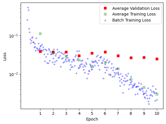
<p>As the labels are continuous values we employ an MSE loss and train using Adam in 10 epochs using batches of size 12 with a validation split of [0.8, 0.2] and a low learning rate of 0.0005.</p>

<h2 id="with-and-without-pretraining">With and without pretraining</h2>
<p>We initialize Google’s vit-base-patch16-224 ViT, replace the classifier and start training. We expected that during fine tuning we would need to carefully consider which layers to freeze and which layers to train. In actuality the naive approach of letting the model adjust all training parameters with the same learning rate works incredibly well converging after essentially one epoch. Therefore we also compared training without pretraining and see, that whilst convergence is a bit slower, the model also learns to capture the correct relationship.</p>

<table>
  <thead>
    <tr>
      <th style="text-align: center">With Pretraining</th>
      <th style="text-align: center">Without Pretraining</th>
    </tr>
  </thead>
  <tbody>
    <tr>
      <td style="text-align: center"><img src="/assets/AutoHDR/pretrained_loss.png" alt="Loss" /></td>
      <td style="text-align: center"><img src="/assets/AutoHDR/unpretrained_loss.png" alt="Loss" /></td>
    </tr>
  </tbody>
</table>

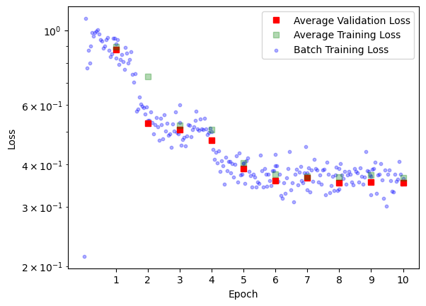
<p>Fig 3: We see that the network pretty much converges after the first epoch until it eventually overfits. We will later try to mitigate the overfitting using label smoothing (see section <a href="#label-smoothing">Label Smoothing</a>). In both cases the final loss is usually around 0.02.</p>

<p>Even though both the pre- and the unpretrained approach both prove very successful, we try to further push the effectiveness of our training. The idea is that a photographer might want to establish a certain style for a single photo shoot. If he now were to edit a small subset of these images in that style, the algorithm can quickly pick up on it and edit the rest. For this however we need to learn effectively on very small datasets. We therefore introduce data augmentation. It will prove similarly effective (see section <a href="#Evaluating-Data-Augmentations">Evaluating Data Augmentations</a>).</p>

<h1 id="falsification-attempt">Falsification Attempt</h1>
<p>Before we pursue data augmentation, we want to better understand the networks almost unreasonable performance. For this, we investigate the training data and the attention heads.</p>

<h2 id="understanding-the-data">Understanding the Data</h2>
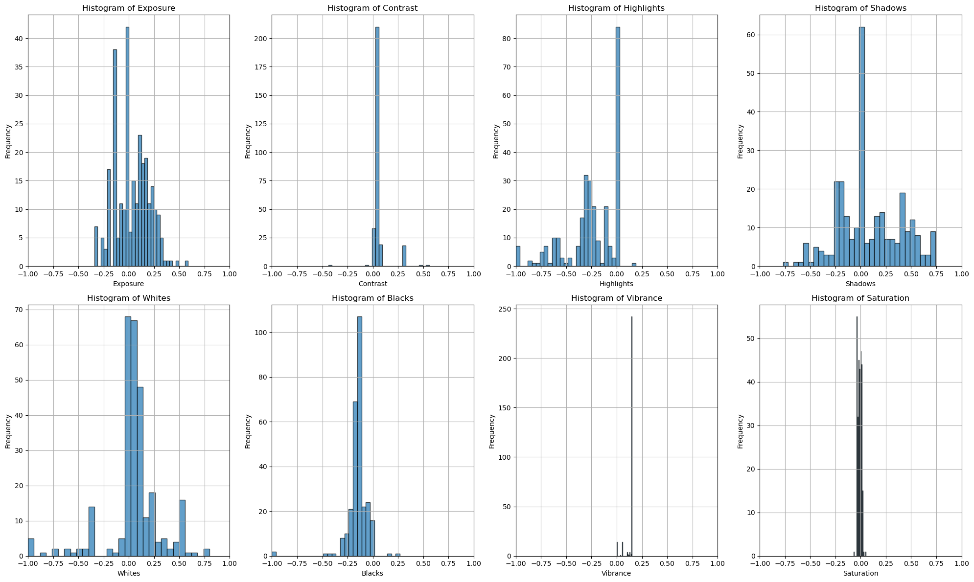
<p>Our first suspicion for the unreasonable performance of our network is, that the data has a very simple structure. It might be possible, that settings such as Exposure or Saturation are essentially the same for all images in the training data. If this were the case, the network could always make a constant guess without being penalized significantly. We are therefore interested in the underlying statistics of the training labels.</p>

<p><img src="/assets/AutoHDR/data_statistics.png" alt="" /></p>

<p>Fig 4: Histogram of the labels in the training dataset</p>

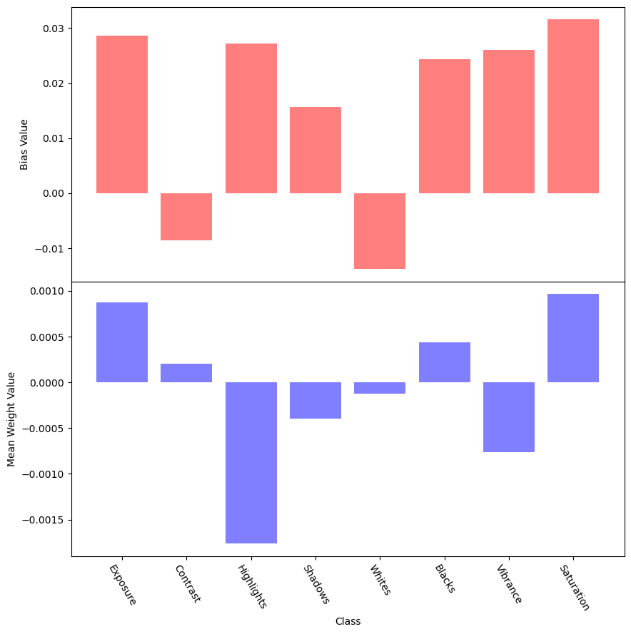
<p>We can clearly see, that some labels are actually quite simple. Saturation and Vibrance almost always have the same value. We expect that the network learns low weights and a bias reflecting the value for these settings.</p>

<p><img src="/assets/AutoHDR/nework_wab.png" alt="" /></p>

<p>Fig 5: In red the bias value for each setting and in blue the average connection strength to that node.</p>

<p>We can see that this hypothesis was false. There is no clear pattern of a specific bias with low connections to it. Keep in mind that due to regularization the average magnitude of incoming connections is also essentially the same for all nodes. Furthermore the plot is anything but constant for different runs indicating that the network is actually responding to the image and not just making a fixed guess.</p>

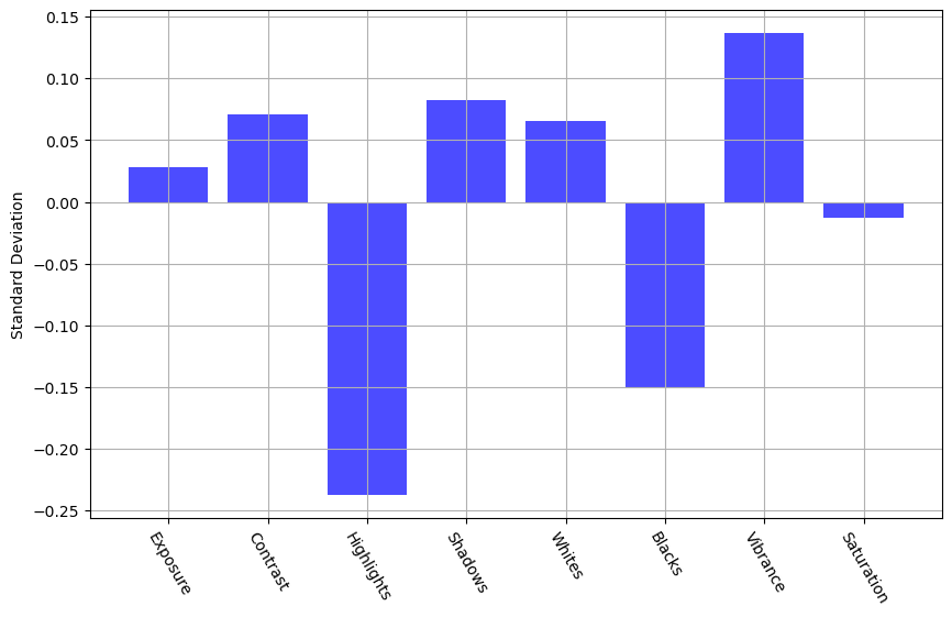
<p>Still, we suspect that a fixed guess might perform quite well. We therefore calculate the mean and standard deviation for each label and construct a simple guesser that picks its label suggestions from a normal distribution with the calculated variance and standard deviation. This guesser considers only the label space and does not take the input image into consideration.</p>

<p><img src="/assets/AutoHDR/mean_and_std.png" alt="" /></p>

<p>Fig 6: Mean and standard deviation of labels in training dataset.</p>

<p>We evaluate this guesser on the validation set with an 80, 20 training - validation split and get a quite consistent loss of ~8%. This is definitely a very good performance considering the guesser did not look at the actual image. It is therefore fair to say that the underlying data is quite homogenous. Still, the random guesser is fortunately outperformed by our ViT model, which consistently achieves loss rates of around ~2%.</p>

<h2 id="understanding-the-attention-heads">Understanding the Attention Heads</h2>
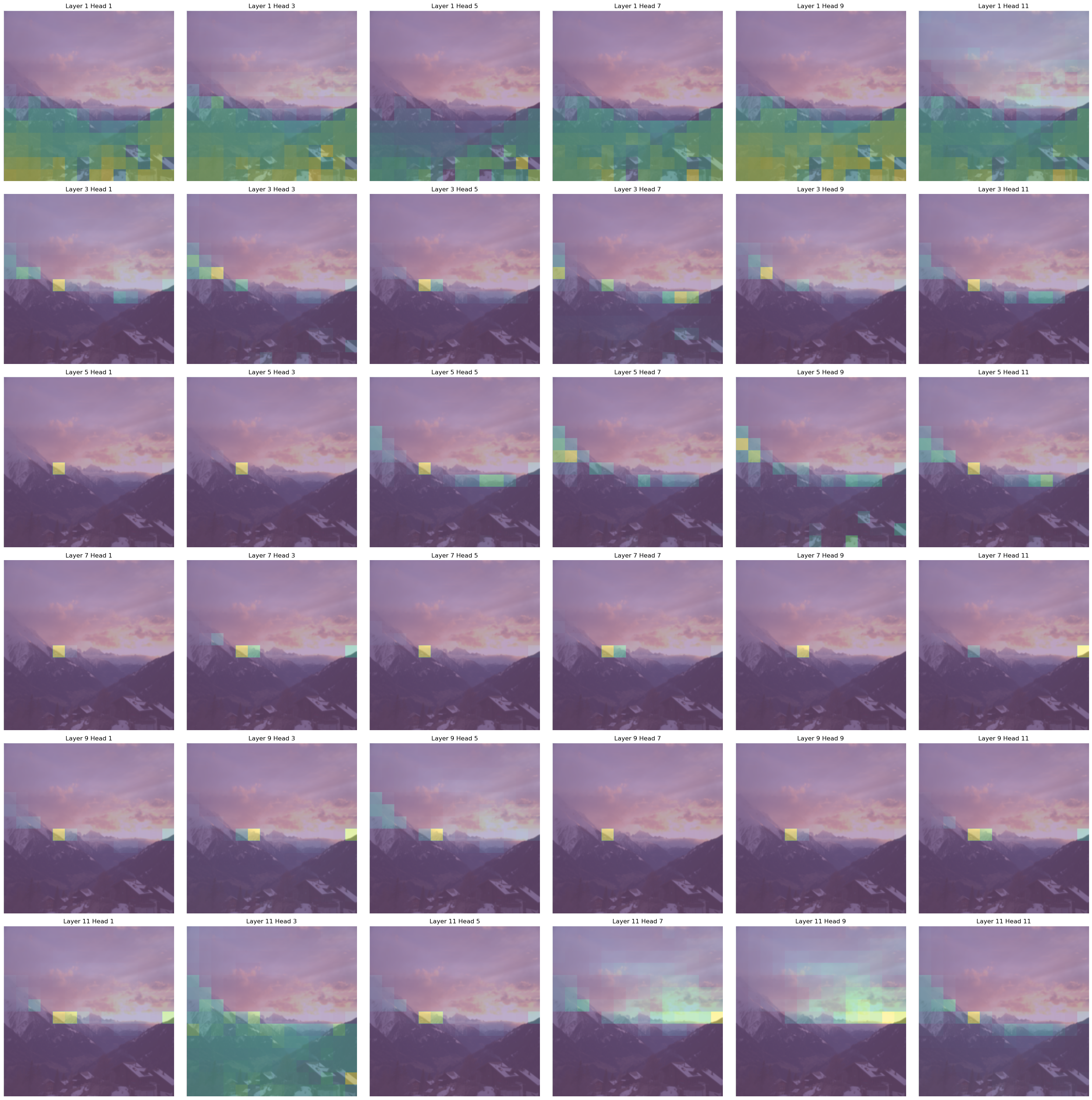
<p>We now seek to understand the attention heads. The hope is that there is a certain structure here, indicating that the network is actually considering different aspects of the input image. As the settings affect the brightness spectrum of the image, we hypothesize that the network should pay attention to shadows, highlights and especially bright light sources (such as the sun).</p>

<p>The ViT works on 16 x 16 tokens plus the cls token in 12 layers using 12 attention heads. For our visualization we highlight the patches that were most attended by each attention head for the cls token. We select a subset of layers and attention maps to make it a bit less convoluted.</p>

<table>
  <thead>
    <tr>
      <th style="text-align: center">Input</th>
      <th style="text-align: center">Attention Maps</th>
    </tr>
  </thead>
  <tbody>
    <tr>
      <td style="text-align: center"><img src="/assets/AutoHDR/attention_input.jpg" alt="Loss" /></td>
      <td style="text-align: center"><img src="/assets/AutoHDR/attention_map.png" alt="Loss" /></td>
    </tr>
  </tbody>
</table>

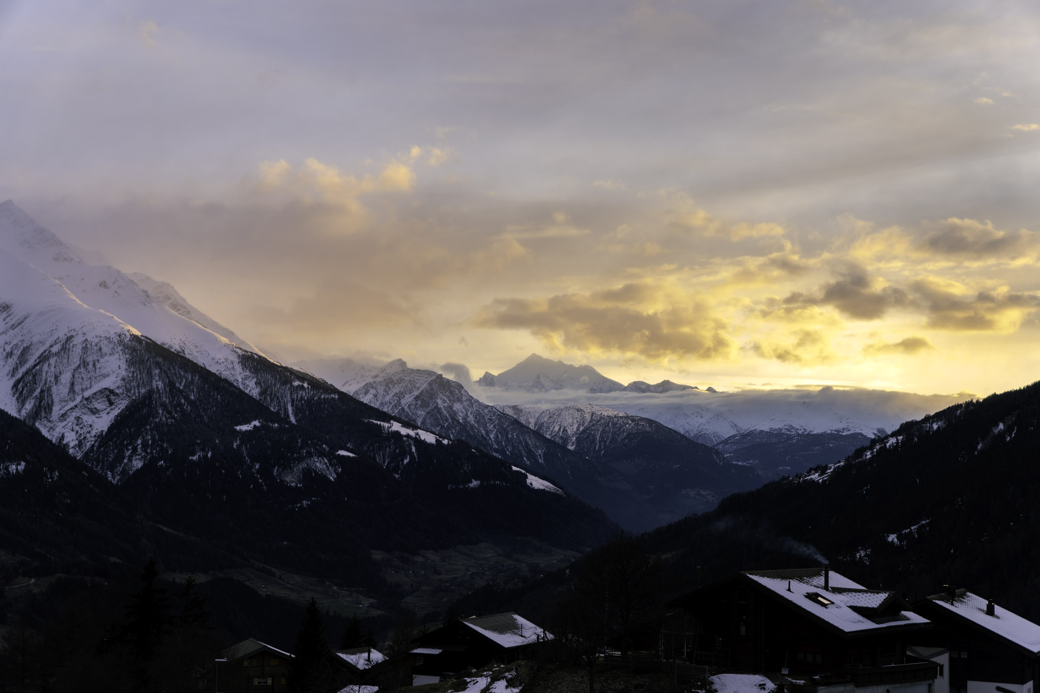
<p>Fig 7: The left image was provided as input to the model, and a subset of attention heads was chosen for the right visualization. We selected every second attention head from every second transformer layer.</p>

<p>Although interpreting attention maps should always be done with a grain of salt, one can tell that heads generally focus on specific brightness regions. This indicates that the network’s suggestion is actually based on the input data as it pays attention to similar areas in the images as a photographer would do when determining brightness settings.</p>

<p>Overall, it is fair to say that even though the underlying data is not too complicated, that is at least not taking obvious escapes such as learning specific values independent of the input.</p>

<h1 id="data-augmentation">Data Augmentation</h1>
<p>Having only a limited amount of labeled data at hand, the generation of synthetic data is a natural approach to improve the sufficiency and diversity of training data. Without such augmention, the model risks overfitting to the training data. The basic idea of augmenting data for training is to introduce minor modifications to the data such that it remains close to the original but exhibits slight variations. For computer vision tasks this means to one changes small aspects of the image while keeping the main content recognizable, e.g. change the background when the task is to detect an object in the foreground. For object detection tasks there are extensive surveys available describing applicable data augmentation methods and providing a numerical analysis of their performance, see [Kumar et al., 2023] and [Yang et al., 2022]. However, our problem sets a different task to solve: we aim to recognize objects and their luminosity relative to the rest of the image. Due to the lack of specific performance data on available methods for this particular problem, we select seven promising basic data augmentation methods and apply them to the problem to evaluate their effectiveness.</p>

<h2 id="data-augmentation-methods">Data Augmentation methods</h2>

<p>We follow the taxonomy of basic data augmentation methods proposed by [Kumar et al., 2023]. For common methods, we use the available implementations provided by torchvision. The last two augmentation methods, not available within any ML framework, were manually implemented based on the respective papers. In the following, we introduce each method that is used in the training process and give a brief heuristic explanation how we think the method could benefit or harm the training.</p>

<h3 id="geometric-image-manipulation">Geometric Image Manipulation</h3>
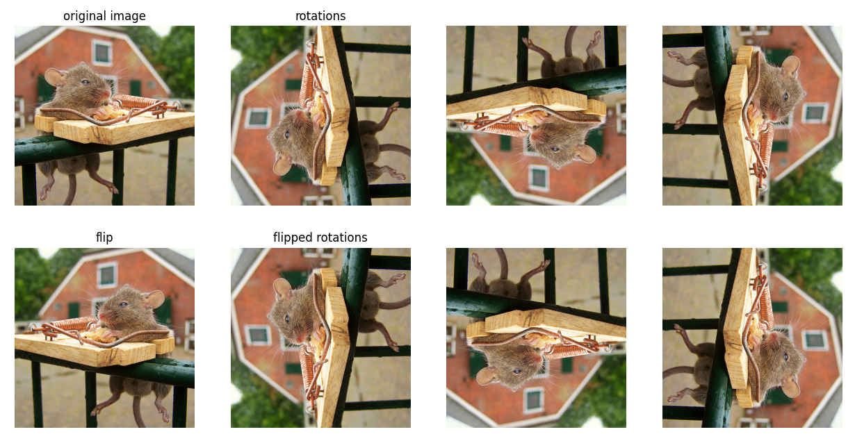
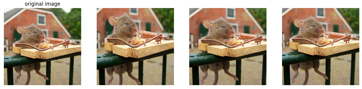
<p><strong>Rotation and Flipping</strong></p>

<p>As a first basic method to augment our training data we use flipping and rotating which preserves the structure and content of the picture, thus minimizing the risk of loosing important information. However, due to its simplicity, it is not able to generate diverse data.</p>

<div class="language-python highlighter-rouge"><div class="highlight"><pre class="highlight"><code><span class="n">imgs</span> <span class="o">=</span> <span class="p">[</span><span class="n">original_img</span><span class="p">]</span>
<span class="n">imgs</span><span class="p">.</span><span class="nf">append</span><span class="p">(</span><span class="n">transforms</span><span class="p">.</span><span class="n">functional</span><span class="p">.</span><span class="nf">hflip</span><span class="p">(</span><span class="n">original_img</span><span class="p">))</span>
<span class="k">for</span> <span class="n">i</span> <span class="ow">in</span> <span class="nf">range</span><span class="p">(</span><span class="mi">3</span><span class="p">):</span>
    <span class="n">imgs</span><span class="p">.</span><span class="nf">append</span><span class="p">(</span><span class="n">transforms</span><span class="p">.</span><span class="n">functional</span><span class="p">.</span><span class="nf">rotate</span><span class="p">(</span><span class="n">original_img</span><span class="p">,</span> <span class="mf">90.0</span><span class="o">*</span><span class="n">i</span><span class="p">))</span>
    <span class="n">imgs</span><span class="p">.</span><span class="nf">append</span><span class="p">(</span><span class="n">transforms</span><span class="p">.</span><span class="n">functional</span><span class="p">.</span><span class="nf">rotate</span><span class="p">(</span><span class="n">transforms</span><span class="p">.</span><span class="n">functional</span><span class="p">.</span><span class="nf">hflip</span><span class="p">(</span><span class="n">original_img</span><span class="p">),</span> <span class="mf">90.0</span><span class="o">*</span><span class="n">i</span><span class="p">))</span>
<span class="nf">plot_images</span><span class="p">(</span><span class="n">imgs</span><span class="p">)</span>
</code></pre></div></div>
<p><img src="/assets/AutoHDR/rotations.png" alt="Rotation and Flipping" /></p>

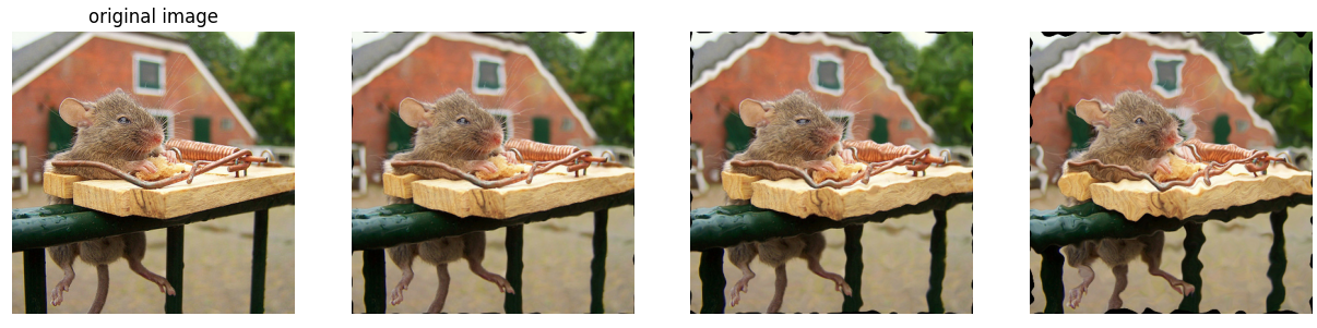
<p><strong>Shearing</strong></p>

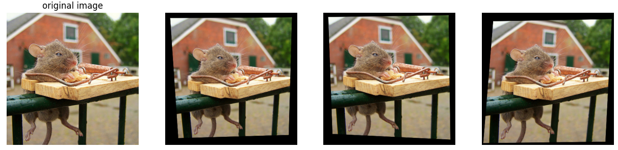
<p>By randomly shearing the picture, we -heuristically speaking- providing the model with different perspectives on the picture. Technically, we are changing the proportion of the objects and their spatial relations. This seems to be a good approach for our task as the luminosity of the picture should not depend on the specific shapes of the objects. However, one drawback is that shearing can generate black, and thus dark, regions on the border of the image.</p>

<div class="language-python highlighter-rouge"><div class="highlight"><pre class="highlight"><code><span class="n">imgs</span> <span class="o">=</span> <span class="p">[</span><span class="n">original_img</span><span class="p">]</span>
<span class="k">for</span> <span class="n">_</span> <span class="ow">in</span> <span class="nf">range</span><span class="p">(</span><span class="mi">3</span><span class="p">):</span>
    <span class="n">transforms</span><span class="p">.</span><span class="nc">RandomPerspective</span><span class="p">(</span><span class="n">distortion_scale</span><span class="o">=</span><span class="mf">0.2</span><span class="p">,</span> <span class="n">p</span><span class="o">=</span><span class="mf">1.0</span><span class="p">)(</span><span class="n">original_img</span><span class="p">)</span>
<span class="nf">plot_images</span><span class="p">(</span><span class="n">imgs</span><span class="p">)</span>
</code></pre></div></div>
<p><img src="/assets/AutoHDR/random_perspective.png" alt="Random Perspective" /></p>

<h3 id="non-geometric-image-manipulation">Non-Geometric Image Manipulation</h3>

<p><strong>Random Cropping and Resize</strong></p>

<p>Randomly cropping a patch from the original picture aims to create a different context for the objects included. We hope to to exclude uninteresting or even distracting elements on the image edges and focus on the main content in the center. Of course this is based on the assumption that we do not loose any crucial information by cropping. As before, the structure and colors of the main content remain untouched.</p>

<div class="language-python highlighter-rouge"><div class="highlight"><pre class="highlight"><code><span class="n">imgs</span> <span class="o">=</span> <span class="p">[</span><span class="n">original_img</span><span class="p">]</span>
<span class="k">for</span> <span class="n">_</span> <span class="ow">in</span> <span class="nf">range</span><span class="p">(</span><span class="mi">3</span><span class="p">):</span>
    <span class="n">size</span> <span class="o">=</span> <span class="p">(</span><span class="n">original_img</span><span class="p">.</span><span class="n">shape</span><span class="p">[</span><span class="mi">1</span><span class="p">],</span><span class="n">original_img</span><span class="p">.</span><span class="n">shape</span><span class="p">[</span><span class="mi">2</span><span class="p">])</span>
    <span class="n">imgs</span><span class="p">.</span><span class="nf">append</span><span class="p">(</span><span class="n">transforms</span><span class="p">.</span><span class="nc">RandomResizedCrop</span><span class="p">(</span><span class="n">size</span><span class="p">,</span> <span class="n">scale</span><span class="o">=</span><span class="p">(</span><span class="mf">0.75</span><span class="p">,</span><span class="mf">1.0</span><span class="p">))(</span><span class="n">original_img</span><span class="p">))</span>
<span class="nf">plot_images</span><span class="p">(</span><span class="n">imgs</span><span class="p">)</span>
</code></pre></div></div>

<p><img src="/assets/AutoHDR/random_cropping.png" alt="Random Cropping and Resize" /></p>

<p><strong>Distortion</strong></p>

<p>Instead of loosing a whole region of the picture and leaving another region completely untouched, we try to add uncertainty to the structure on the whole picture. By adding distortion we reduce the sharpness of the edges of the objects. Since the task possibly involves detecting regions of varying light intensity, which are usually not separated by sharp edges, this approach hopefully supports the model training.</p>

<div class="language-python highlighter-rouge"><div class="highlight"><pre class="highlight"><code><span class="n">imgs</span> <span class="o">=</span> <span class="p">[</span><span class="n">original_img</span><span class="p">]</span>
<span class="k">for</span> <span class="n">i</span> <span class="ow">in</span> <span class="nf">range</span><span class="p">(</span><span class="mi">3</span><span class="p">):</span>
    <span class="n">imgs</span><span class="p">.</span><span class="nf">append</span><span class="p">(</span><span class="n">transforms</span><span class="p">.</span><span class="nc">ElasticTransform</span><span class="p">(</span><span class="n">alpha</span><span class="o">=</span><span class="p">[</span><span class="mf">50.</span><span class="o">+</span><span class="mf">50.</span><span class="o">*</span><span class="n">i</span><span class="p">])(</span><span class="n">original_img</span><span class="p">))</span>
<span class="nf">plot_images</span><span class="p">(</span><span class="n">imgs</span><span class="p">)</span>
</code></pre></div></div>
<p><img src="/assets/AutoHDR/distortion.png" alt="Distortion" /></p>

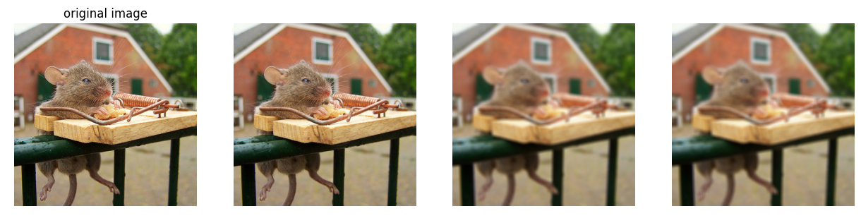
<p><strong>Gaussian blurring</strong></p>

<p>With the same heuristics as before we apply a gaussian blur to the whole picture. As the object itself stays untouched in terms of shape and luminosity, this augmentation method should also go along well with our training task.</p>

<div class="language-python highlighter-rouge"><div class="highlight"><pre class="highlight"><code><span class="n">imgs</span> <span class="o">=</span> <span class="p">[</span><span class="n">original_img</span><span class="p">]</span>
<span class="k">for</span> <span class="n">_</span> <span class="ow">in</span> <span class="nf">range</span><span class="p">(</span><span class="mi">3</span><span class="p">):</span>
    <span class="n">imgs</span><span class="p">.</span><span class="nf">append</span><span class="p">(</span><span class="n">transforms</span><span class="p">.</span><span class="nc">GaussianBlur</span><span class="p">(</span><span class="n">kernel_size</span><span class="o">=</span><span class="p">(</span><span class="mi">9</span><span class="p">,</span><span class="mi">9</span><span class="p">),</span> <span class="n">sigma</span><span class="o">=</span><span class="p">(</span><span class="mf">0.1</span><span class="p">,</span><span class="mf">5.0</span><span class="p">))(</span><span class="n">original_img</span><span class="p">))</span>
<span class="nf">plot_images</span><span class="p">(</span><span class="n">imgs</span><span class="p">)</span>
</code></pre></div></div>
<p><img src="/assets/AutoHDR/gaussian_blur.png" alt="Gaussian Blur" /></p>

<h3 id="image-erasing">Image Erasing</h3>
<p>By taking out parts of the image one hopefully drops out dominant regions that could prevent the model from learning less sensitive information beforehand. Without them, we enhance a more robust model. However, these methods may inadvertently remove important parts relevant to our task. Known examples for Image Erasing are random erasing, cutout or hide-and-seek, see [Kumar et al., 2023].
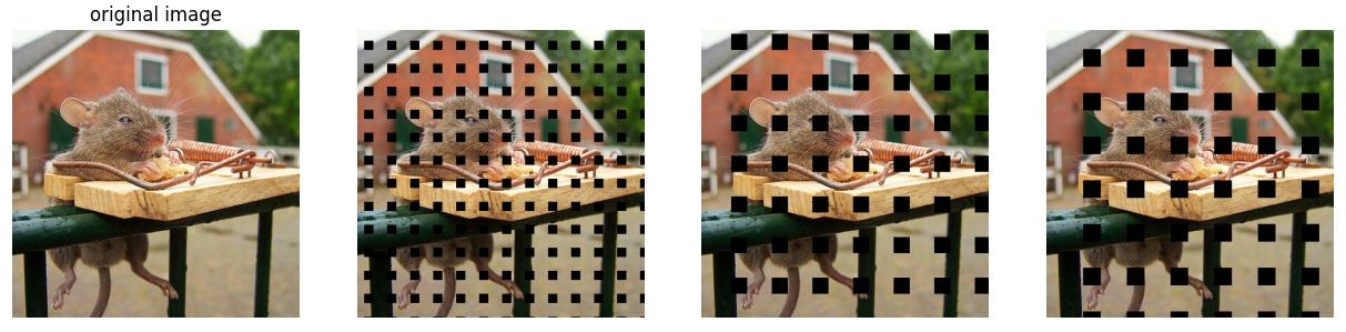
<strong>Gridmask deletion</strong>
The perviously mentioned dropout methods have two main problems for our task. Since they delete a continuous region or an excessive amount of data they tend to delete important parts for our task, i.e. as our problem cannot be fully reduced to object identification we cannot be sure which part of the background is important. To overcome these problems, in [Chen et al., 2020] the so-called GridMask data augmentation method is introduced.
Here a grid consisting of small mask units is created, where the parameter $r\in (0,1)$ denotes the ratio of the shorter visible edge in a unit, and the unit size $d=\text{random}(d_{min},d_{max})$ is randomly chosen. Lastly the distances $\delta_x,\,\delta_y\in (0,d-1)$ between the first intact unit and the boundary of the image are also chosen randomly. For these parameters a grid mask is created which is later applied to the actual image.</p>
<div class="language-python highlighter-rouge"><div class="highlight"><pre class="highlight"><code><span class="k">def</span> <span class="nf">grid_mask</span><span class="p">(</span><span class="n">shape</span><span class="p">,</span> <span class="n">r</span><span class="p">,</span> <span class="n">d</span><span class="p">,</span> <span class="n">delta_x</span><span class="p">,</span> <span class="n">delta_y</span><span class="p">):</span>
    <span class="n">mask</span> <span class="o">=</span> <span class="n">torch</span><span class="p">.</span><span class="nf">ones</span><span class="p">(</span><span class="n">shape</span><span class="p">)</span>
    <span class="n">ones_l</span> <span class="o">=</span> <span class="nf">round</span><span class="p">(</span><span class="n">r</span><span class="o">*</span><span class="n">d</span><span class="p">)</span>
    <span class="n">zeros_l</span> <span class="o">=</span> <span class="n">d</span><span class="o">-</span><span class="n">ones_l</span>
    <span class="n">start_x</span><span class="p">,</span> <span class="n">start_y</span> <span class="o">=</span> <span class="n">delta_x</span><span class="p">,</span> <span class="n">delta_y</span>

    <span class="k">while</span> <span class="n">start_x</span><span class="o">&lt;=</span> <span class="n">shape</span><span class="p">[</span><span class="mi">1</span><span class="p">]:</span>
        <span class="n">end_x</span> <span class="o">=</span> <span class="nf">min</span><span class="p">(</span><span class="n">start_x</span><span class="o">+</span><span class="n">zeros_l</span><span class="p">,</span> <span class="n">shape</span><span class="p">[</span><span class="mi">1</span><span class="p">])</span>
        
        <span class="k">while</span>  <span class="n">start_y</span><span class="o">&lt;=</span><span class="n">shape</span><span class="p">[</span><span class="mi">2</span><span class="p">]:</span>
            <span class="n">end_y</span> <span class="o">=</span> <span class="nf">min</span><span class="p">(</span><span class="n">start_y</span><span class="o">+</span><span class="n">zeros_l</span><span class="p">,</span> <span class="n">shape</span><span class="p">[</span><span class="mi">2</span><span class="p">])</span>
            <span class="n">mask</span><span class="p">[:,</span><span class="n">start_x</span><span class="p">:</span><span class="n">end_x</span><span class="p">,</span> <span class="n">start_y</span><span class="p">:</span><span class="n">end_y</span><span class="p">]</span> <span class="o">=</span> <span class="mi">0</span>
            <span class="n">start_y</span> <span class="o">=</span> <span class="n">end_y</span> <span class="o">+</span> <span class="n">ones_l</span>
        <span class="n">start_x</span> <span class="o">=</span> <span class="n">end_x</span> <span class="o">+</span> <span class="n">ones_l</span>
        <span class="n">start_y</span> <span class="o">=</span> <span class="n">delta_y</span>   

    <span class="k">return</span> <span class="n">mask</span>
</code></pre></div></div>
<p>The experiment results in [Chen et al., 2020] show a higher accuracy when training a ResNet under the usage of GridMask compared to standard image erasing methods on the ImageNet Dataset.</p>
<div class="language-python highlighter-rouge"><div class="highlight"><pre class="highlight"><code><span class="n">imgs</span> <span class="o">=</span> <span class="p">[</span><span class="n">original_img</span><span class="p">]</span>
<span class="k">for</span> <span class="n">_</span> <span class="ow">in</span> <span class="nf">range</span><span class="p">(</span><span class="mi">3</span><span class="p">):</span>
    <span class="n">imgs</span><span class="p">.</span><span class="nf">append</span><span class="p">(</span><span class="nf">gridmask_deletion</span><span class="p">(</span><span class="n">original_img</span><span class="p">,</span> <span class="n">r</span><span class="o">=</span><span class="mf">0.6</span><span class="p">,</span> <span class="n">d_min</span><span class="o">=</span><span class="mi">30</span><span class="p">,</span> <span class="n">d_max</span><span class="o">=</span><span class="mi">70</span><span class="p">))</span>
<span class="nf">plot_images</span><span class="p">(</span><span class="n">imgs</span><span class="p">)</span>
</code></pre></div></div>
<p><img src="/assets/AutoHDR/grid_mask.png" alt="Gridmask deletion" /></p>

<h3 id="advanced-image-manipulation">Advanced Image Manipulation</h3>
<p><strong>Local Rotation</strong>
This method is introduced in [Kim et al., 2021] as part of a collection of local augmentation methods. In this case local rotation can be seen as a further development of global rotation. It was developed as an augmentation method for CNNs. As CNNs are biased to local features which is a disadvantage for generalization, we cut the picture in four patches that are then randomly rotated and glued together. In this way we might break up some strong local features, which should be advantageous for our problem that is mainly interested in the global luminosity. In [Kim et al., 2021] it is stated that the CIFAR100 test accuracy for a ResNet is superior if local rotation is used compared to global rotation.</p>

<p>The local rotation introduces significant discontinuities into the image. This might be detrimental for tasks such as object recognition, as permutations might lead to objects being ripped apart. But for our task the locations should not destroy the training data, as the global illumination of the image stays essentially the same.</p>

<div class="language-python highlighter-rouge"><div class="highlight"><pre class="highlight"><code><span class="n">imgs</span> <span class="o">=</span> <span class="p">[</span><span class="n">original_img</span><span class="p">]</span>
<span class="k">for</span> <span class="n">_</span> <span class="ow">in</span> <span class="nf">range</span><span class="p">(</span><span class="mi">3</span><span class="p">):</span>
    <span class="n">imgs</span><span class="p">.</span><span class="nf">append</span><span class="p">(</span><span class="nf">local_rotation</span><span class="p">(</span><span class="n">original_img</span><span class="p">))</span>
<span class="nf">plot_images</span><span class="p">(</span><span class="n">imgs</span><span class="p">)</span>
</code></pre></div></div>

<p><img src="/assets/AutoHDR/local_rotation.png" alt="Local Rotation" /></p>

<h1 id="label-smoothing">Label smoothing</h1>
<p>Label smoothing tackles the problem that the labels in the dataset are noisy. This noise is especially relevant in our dataset, as in the artistic process of editing a photo, there are no right or wrong settings. Furthermore if you were to give a photographer the same photo to edit twice, we are quite certain, that the result would not be the same.</p>

<p>[Szegedy et al., 2016] introduces label smoothing for classification tasks, by assuming that for a small $\varepsilon&gt;0$ the training set label is correct with only probability $1-\varepsilon$ and incorrect otherwise. We now strive to come up with a similar mechanism for regression tasks reflecting the lack of a correct choice in the task.</p>

<h2 id="label-smoothing-methods">Label smoothing methods</h2>
<p>As there are no discrete classes but continuous values we work with two different approaches to smooth the labels. In the first approach, given a sequence of training labels, we apply a moving average across the dataset for each label dimension. For the second approach, we add random gaussian noise to each value, based on the assumptions that whilst the label does not need the exact value as given in the training data, it should still be roughly in the same ballpark. The implementation details of these smoothing methods are provided below. We hope, that this smoothing decreases overfitting.</p>
<div class="language-python highlighter-rouge"><div class="highlight"><pre class="highlight"><code><span class="k">def</span> <span class="nf">smoothing</span><span class="p">(</span><span class="n">labels</span><span class="p">,</span> <span class="n">method</span><span class="o">=</span><span class="sh">'</span><span class="s">moving_average</span><span class="sh">'</span><span class="p">,</span> <span class="n">window_size</span><span class="o">=</span><span class="mi">5</span><span class="p">,</span> <span class="n">sigma</span><span class="o">=</span><span class="mi">2</span><span class="p">):</span>
    <span class="k">if</span> <span class="n">method</span> <span class="o">==</span> <span class="sh">'</span><span class="s">moving_average</span><span class="sh">'</span><span class="p">:</span>
        <span class="c1"># Apply moving average smoothing
</span>        <span class="k">if</span> <span class="n">window_size</span> <span class="o">&gt;</span> <span class="mi">0</span><span class="p">:</span>
            <span class="n">smoothed_labels</span> <span class="o">=</span> <span class="n">np</span><span class="p">.</span><span class="nf">convolve</span><span class="p">(</span><span class="n">labels</span><span class="p">,</span> <span class="n">np</span><span class="p">.</span><span class="nf">ones</span><span class="p">(</span><span class="n">window_size</span><span class="p">)</span><span class="o">/</span><span class="n">window_size</span><span class="p">,</span> <span class="n">mode</span><span class="o">=</span><span class="sh">'</span><span class="s">same</span><span class="sh">'</span><span class="p">)</span>
        <span class="k">else</span><span class="p">:</span> 
            <span class="n">smoothed_labels</span> <span class="o">=</span> <span class="n">labels</span>
    <span class="k">elif</span> <span class="n">method</span> <span class="o">==</span> <span class="sh">'</span><span class="s">gaussian</span><span class="sh">'</span><span class="p">:</span>
        <span class="c1"># Apply Gaussian smoothing
</span>        <span class="n">smoothed_labels</span> <span class="o">=</span> <span class="n">scipy</span><span class="p">.</span><span class="n">ndimage</span><span class="p">.</span><span class="nf">gaussian_filter1d</span><span class="p">(</span><span class="n">labels</span><span class="p">,</span> <span class="n">sigma</span><span class="o">=</span><span class="n">sigma</span><span class="p">)</span>
    <span class="k">else</span><span class="p">:</span>
        <span class="k">raise</span> <span class="nc">ValueError</span><span class="p">(</span><span class="sh">"</span><span class="s">Unsupported smoothing method</span><span class="sh">"</span><span class="p">)</span>
    <span class="k">return</span> <span class="n">smoothed_labels</span>
</code></pre></div></div>

<h1 id="evaluating-data-augmentations">Evaluating Data Augmentations</h1>
<p>For evaluation we iterate over every possible augmentation method and select hyperparameters such that the amount of data is increased by factor eight. This value is chosen since it is the maximal factor using flipping and rotation and we want to obtain comparable results. Each augmentation method is combined with either no label smoothing, moving average or gaussian smoothing. Overall we obtain 21 possible combinations of label smoothing and data augmentation. For each of them the model is trained 30 times with a 0.05/0.95 training/validation split, simulating extreme data scarcity. We average the validation losses across all 30 models.</p>

<iframe src="/assets/AutoHDR/interactive_plot.html" style="width: 100%; height: 400px; border: none;"></iframe>

<p>Fig 8: Comparison average epoch validation losses of different augmentations.</p>

<p>What immediately catches the eye, is that data augmentation in principle has a positive impact on the model’s performance. Sobering, however is the impact of label smoothing. Without data augmentation it even seems to have a negative effect. At least on augmented data the models that are trained on smoothed data perform better than the ones with untreated labels. This suggests the assumption that having a certain amount of training data available is necessary for label smoothing to work. But this question is up to another evaluation since the observed effect is not pronounced.</p>

<p>It is hard to say what augmentation works the best. It is however fair to say, that smoothing does seem to help with the validation error, possibly due to reduced overfitting. Furthermore we are inclined to say, that image erasing performs the worst. This may be because the deleted spots are registered as shadows, messing up the algorithms understanding of the scenes lighting. Both effects are however not strong and require further inquiry.</p>

<h1 id="conclusion">Conclusion</h1>
<p>Our algorithm manages to find a photographer’s editing style from an extremely small dataset (15-20 images) allowing a photographer to edit a subset of a photo shoot and let the algorithm decide the rest. The algorithm also learns to match editing styles, that are typical for HDR photography solving our original goal. This greatly reduces the time needed to edit photos, mitigating one of the less fun aspects of photography.</p>
<h1 id="references">References</h1>
<p>[Chen et al., 2020] Chen, Pengguang, et al. “Gridmask data augmentation.” arXiv preprint arXiv:2001.04086 (2020).</p>

<p>[Kim et al., 2021] Kim, Youmin, AFM Shahab Uddin, and Sung-Ho Bae. “Local augment: Utilizing local bias property of convolutional neural networks for data augmentation.” IEEE Access 9 (2021).</p>

<p>[Kumar et al., 2023] Kumar, Teerath, et al. “Image data augmentation approaches: A comprehensive survey and future directions.” arXiv preprint arXiv:2301.02830 (2023).</p>

<p>[Szegedy et al., 2016] Szegedy, Christian, et al. “Rethinking the inception architecture for computer vision.” Proceedings of the IEEE conference on computer vision and pattern recognition. (2016).</p>

<p>[Yang et al., 2022] Yang, Suorong, et al. “Image data augmentation for deep learning: A survey.” arXiv preprint arXiv:2204.08610 (2022).</p>

<p>[Dosovitskiy et al., 2020] Dosovitskiy, Alexey et al. “An Image is Worth 16x16 Words: Transformers for Image Recognition at Scale.” ArXiv abs/2010.11929 (2020): n. pag.</p>]]></content><author><name>Stanislaus Stein</name><email>stanislaussteinvk@gmail.com</email></author><category term="blog" /><summary type="html"><![CDATA[Adapting a Vision Transformer to find image rendering settings suitable for HDR image editing from small training datasets.]]></summary></entry><entry><title type="html">Exploring Skip Connections in MLPs</title><link href="https://stani-stein.com//blog/A-ResNet-Investigation/" rel="alternate" type="text/html" title="Exploring Skip Connections in MLPs" /><published>2024-04-01T00:00:00+02:00</published><updated>2024-04-01T00:00:00+02:00</updated><id>https://stani-stein.com//blog/A-ResNet-Investigation</id><content type="html" xml:base="https://stani-stein.com//blog/A-ResNet-Investigation/"><![CDATA[<h1 id="abstract">Abstract</h1>
<p>This blog post investigates the behaviour of an MLP, where every layer has a skip connection to the last hidden layer. We will see, that such networks tend to perform all relevant computations in early layers, while latter layers tend to learn the identity. One might say that the network learns the most efficient depth. I hypothesize that this is related to the optimal network architecture for a given dataset, but also refute this hypothesis. Further investigation is still needed.</p>

<h1 id="motivation">Motivation</h1>
<p>Skip connections have proven to be one of the most important concepts in deep learning, as they allow for easy gradient flow during training. One has to distinguish between two different kind of skip connections. The first kind, often called V1 skips before the final non linearity of the residual block. Mathematically speacing we have</p>

\[x' = \sigma (F(x) + Wx ),\]

<p>where x is the input of the residual block, $\sigma()$, the chosen non linearity and $F(x)$ the processing of the block. The processing can range from a simple linear transformation up to a multi head attention block. The linear transformation $W$ may be needed to ensure equal dimensionality. We denote the output of the residual block by $x’$.</p>

<p>The second kind of residual block, often called V2, performs the skip after the final non linearity of the residual block. The expression thus becomes</p>

\[x' = \sigma (F(x)) + Wx .\]

<p>An illustration of such a skip connection is given by</p>

<p><img src="/assets/images/ResNetV2.jpg" alt="ResNet" /></p>

<p>We now modify the structure of V2 blocks. Instead of integrating separate blocks into an MLP, we throw everything together into a sort of telescope structure and allow each layer to skip to the last hidden layer. The following illustrates this approach</p>

<p><img src="/assets/images/SkipNetV2.jpg" alt="ResNet" /></p>

<h1 id="implementation">Implementation</h1>
<p>We simplify the structure by maintaining uniform width across all hidden layers. We can thus use the identity for the skip. The forward pass is defined as follows</p>

<figure class="highlight"><pre><code class="language-python" data-lang="python"><table class="rouge-table"><tbody><tr><td class="gutter gl"><pre class="lineno">1
2
3
4
5
6
7
8
9
10
11
12
13
14
15
16
17
18
19
20
21
22
23
24
25
</pre></td><td class="code"><pre><span class="k">def</span> <span class="nf">forward</span><span class="p">(</span><span class="n">self</span><span class="p">,</span> <span class="n">x</span><span class="p">,</span> <span class="n">layers_disabled</span><span class="o">=</span><span class="bp">None</span><span class="p">):</span>
    <span class="c1"># Initialize array that disables skips during inference, default is [None] * depth
</span>    <span class="c1"># i.e. no skip connections are disabled
</span>    <span class="k">if</span> <span class="n">layers_disabled</span> <span class="ow">is</span> <span class="bp">None</span><span class="p">:</span>
        <span class="n">layers_disabled</span> <span class="o">=</span> <span class="p">[</span><span class="bp">False</span><span class="p">]</span><span class="o">*</span><span class="n">self</span><span class="p">.</span><span class="n">depth</span>
    
    <span class="c1"># Zipping layers and layers_disabled array
</span>    <span class="n">layers_out</span> <span class="o">=</span> <span class="p">[]</span>
    <span class="k">for</span> <span class="n">idx</span><span class="p">,</span> <span class="p">(</span><span class="n">layer</span><span class="p">,</span> <span class="n">disabled</span><span class="p">)</span> <span class="ow">in</span> <span class="nf">enumerate</span><span class="p">(</span><span class="nf">zip</span><span class="p">(</span><span class="n">self</span><span class="p">.</span><span class="n">layers</span><span class="p">,</span> <span class="n">layers_disabled</span><span class="p">)):</span>
    
        <span class="c1"># Feed forward through layers
</span>        <span class="n">x</span> <span class="o">=</span> <span class="nf">layer</span><span class="p">(</span><span class="n">x</span><span class="p">)</span>
        
        <span class="c1"># If skip_connections is enabled and the layer is not disabled, save the value
</span>        <span class="k">if</span> <span class="n">self</span><span class="p">.</span><span class="n">skip_connections</span> <span class="ow">and</span> <span class="ow">not</span> <span class="n">disabled</span><span class="p">:</span>
            <span class="n">layers_out</span><span class="p">.</span><span class="nf">append</span><span class="p">(</span><span class="n">x</span><span class="p">)</span>
    
    <span class="c1"># If skip_connections is enabled, add the sum of layers_out to x
</span>    <span class="k">if</span> <span class="n">self</span><span class="p">.</span><span class="n">skip_connections</span><span class="p">:</span>
        <span class="n">x</span> <span class="o">=</span> <span class="n">x</span> <span class="o">+</span> <span class="nf">sum</span><span class="p">(</span><span class="n">layers_out</span><span class="p">)</span>
    
    <span class="c1"># output layer
</span>    <span class="n">y</span> <span class="o">=</span> <span class="n">self</span><span class="p">.</span><span class="nf">output_layer</span><span class="p">(</span><span class="n">x</span><span class="p">)</span>
    
    <span class="k">return</span> <span class="n">y</span> 
</pre></td></tr></tbody></table></code></pre></figure>

<p>I save the layer outputs in line 16. The actual skip happens in line 20. The class is written in such a way that I can disable skips during inference, but not during training. This is done via the (misslabled) “layers_disabled” array that is checked in line 15. In addition I can also initialise a network without any skips by setting “self.skip_connections” to False. This results in a usual MLP. What I can not do is to only train with selective skips.</p>

<h1 id="analysis">Analysis</h1>
<p>This implementation allowes me to analyse the effect of the skip connections on the networks performance. I quickly noted, that disabling skip connections in the latter half has little effect on the accuracy, whilst disabling skip connections in the front half lead to the network realizing a constant function almost immediately. Figure 1 shows then effect. In other words: I can skip the later layers without issues, but if I don’t allow the first layers to skip to the end, everything breaks.</p>

<p><img src="/assets/images/realized_comparison_resnet.png" alt="" />
<em>Figure 1: A modified ResNet of depth 50, width 64 with ReLU activation. The network was trained with all skip connections enabled. The blue line shows the realized function with all skip connections, the green line shows the realized function if only the first 25 skips are used, the orange line shows the realized function if only the last 25 skips are used.</em></p>
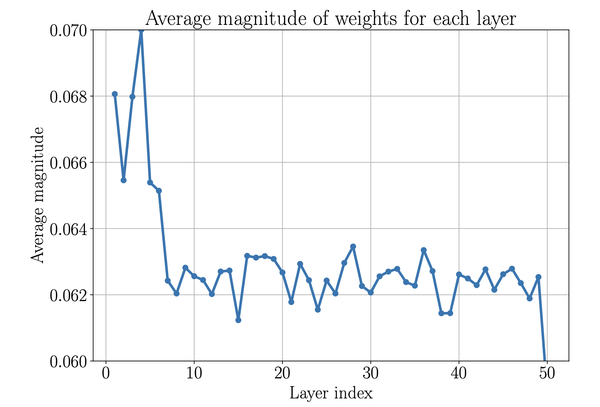
<p>The irrelevance of the latter skip connections indicates to me, that the network learns to express a constant zero function in the tail end. If this is the case, then it doesn’t matter if we allow a skip in the tail or not, as $0 + 0 = 0$. If this scenario is the accurate, it would also mean, that early skips are highly relevant, as if they are suppressed, then the network would have to push everything through these constant zero functions, immediately zeroing out the resulting function. Such behaviour would support the behaviour seen.</p>

<h2 id="investigating-layer-activity">Investigating Layer Activity</h2>
<p>To support this hypothesis I looked at the average magnitude of the weights of different layers, the idea being, that if it is close to zero, that the layer essentially realizes the zero function and I conjuction with an earlier skip essentially the identity. I ran a simple average over each weight matrix and plotted them by layer. This is shown in figure 2.</p>

<p><img src="/assets/images/magnitude_modified_resnet.png" alt="" />
<em>Figure 2: Average magnitude of the weights the hidden layers of the modified V2 model. We can see, that the most significant processing happens in the first five to seven layers. Layer 50 is usually an outlier, as it receives all the skip connections including one from itself.</em></p>
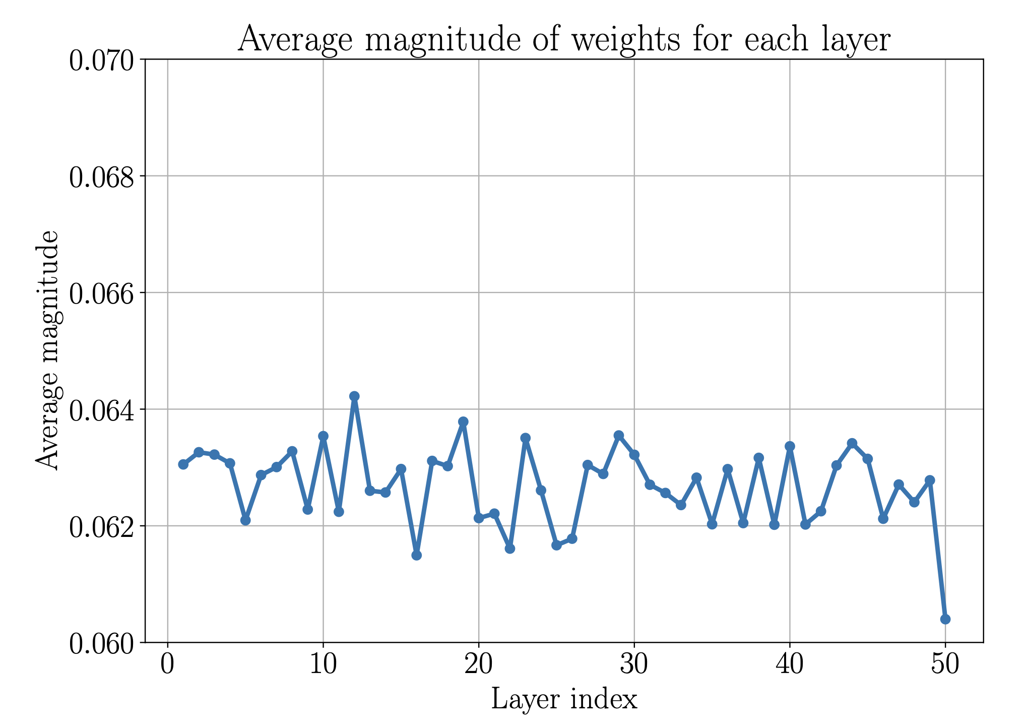
<p>Just as a sanity check we compare this to a normal V2 model and get the layer activity seen in figure 3.</p>

<p><img src="/assets/images/magnitude_normal_resnet.png" alt="" />
<em>Figure 3: Average magnitude of the hidden layers of a ResNet V2. Here the processing seems to be equally distributed among the layers.</em></p>

<p>Both networks are of depth 50 and width 64, use ReLU activations and were trained on the same data set for 2000 epochs using Adam.</p>

<h2 id="investigating-self-truncation">Investigating Self Truncation</h2>
<p>My idea now was, that the skip connections essentially allow the network to always truncate itself. Every layer in essence acts as the final hidden layer, which could mean that they compete in some way. Thus if the first five to seven layers out compete the others, they may have some inherent advantage. This may extend to normal MLPs as well, in the sense that if I make my network too deep, I might not be able to utilize that advantage, as the later layers will make the training of the first layers harder.</p>

<p>I did some more analysis by disabling selective layers, which again showed the importance of the first seven layers and thus formulated my loose hypothesis: “The activity of the first layers reflects their learning efficiency compared to later layers”. Finally I wanted to see if this could also be seen in normal MLPs. To test this I initialized MLPs with the same width of 64, ReLU activations with depth ranging from 2 to 50 and trained these networks using the same training routine as before on the same training data in 100 epochs. To quantify the error I employed a Monte-Carlo method by generating 1000 random points $x_i \in \operatorname{supp}(\text{Training Data})$ and calculating</p>

\[\text{error approximation} = \frac{1}{1000}\sum_{i=1}^{1000} \left( \sin(x_i) - \Phi_\text{depth}(x_i) \right)^2,\]

<p>where $\Phi_\text{depth}$ is the inference of an MLP with specified depth. The results are shown in figure 4.</p>

<p><img src="\assets\images\error_MLPs_100.png" alt="" />
<em>Figure 4: Monte-Carlo error approximation for ReLU MLPs of different depth. Each network was given the same training dataset and trained in the same number of epochs. One can clearly see, how networks between depth 8-13 seem to have an advantage in this rather short training routine.</em></p>

<p>This does not quite support my Hypothesis, as the gains start after the first seven layers. Maybe the hight activity indicates, that the layers are actually needed or maybe it is just an insignificant anomaly of the modified ResNet. Testing this hypothesis on different network sizes with different tasks is needed to be more confident in the hypothesis.</p>

<p>I want to make two remarks on figure 4:</p>
<ul>
  <li>One can nicely see the depth at which the network gets too deep to be trained without skip connections</li>
  <li>The plot is highly dependant upon the training amount. If we increase the epochs we can make shallow networks with comparable accuracy to medium sized networks.</li>
</ul>

<h1 id="further-ideas">Further Ideas</h1>
<p>The first weight update should be highly dependant on the chosen weight initialization scheme. Let’s assume for a second, that the network is initialized with zero bias and the identity for the weights. In this case each layer gets exactly the input data and directly escapes to the last layer. Therefore they are all identical and should receive exactly the same gradient. This changes in every subsequent weight update, as layers no longer realize the identity. The question is now, if the early layers now carry a larger gradient. This seems a bit counter intuitive, as any change made to early layers should also effect the last layer through every subsequent skip. Latter layers in contrast have ever less skips to influence this layer and should thus receive larger gradients to make up for this reduced effect strength. It might be interesting to initialize the network as described above and to investigate the gradient behaviour.</p>

<p>Now lets assume He initialization for the network. In this case each layer immediately receives a different input and therefore the first gradient should be unique for each layer. In other words: We immediately are in this chaotic behaviour. The question is now if the first weight update is of high importance. These considerations however still do not explain why we see the drop of in weight magnitude throughout the layers. It might also be interesting to build a very small network and investigate each weight update individually to better understand the drift of the latter layers to the zero function.</p>

<p>As far as I’m aware PyTorch initializes ReLU networks using He initialization. Therefore the answer to this drift should not be found in the first gradient update. I leave the investigation here for now and might return to it later.</p>]]></content><author><name>Stanislaus Stein</name><email>stanislaussteinvk@gmail.com</email></author><category term="blog" /><summary type="html"><![CDATA[Investigating the Behaviour of an MLP under a novel Skip Configuration.]]></summary></entry></feed>