Visualizing Stem Cell Reprogramming

Comparing variational to non variational Autoencoder

The following visualizes the latent space of an Autoencoder trained on the Schiebinger Data. We can clearly see the cell undifferentiation paths.

Fig 1: Umap of the Latent Space generated by the Autoencoder. Colors are based on Leiden Clustering

We now make the Autoencoder variational and weigh the KL loss with a factor of 0 in the first epoch, 1/150 in the second and 2/150 in the third. We can clearly see how even such a small KL term heavily encourages the network to spread out in the latent space. We lose the clear paths we’ve seen before.

Fig 2: Umap of the Latent Space generated by the Variational Autoencoder. Colors are based on Leiden Clustering

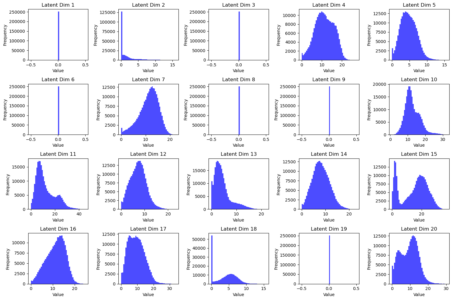
The second thing that is interesting about the non variational Autoencoder are the histograms of the individual latent dimensions across the cells:

Fig 3: Latent Histograms of Autoencoder

We can see, that the model learns to keep some dimensions constant zero. This might indicate, that the underlying data manifold only has around 15 dimensions. Obviously this varies from run to run somewhat.

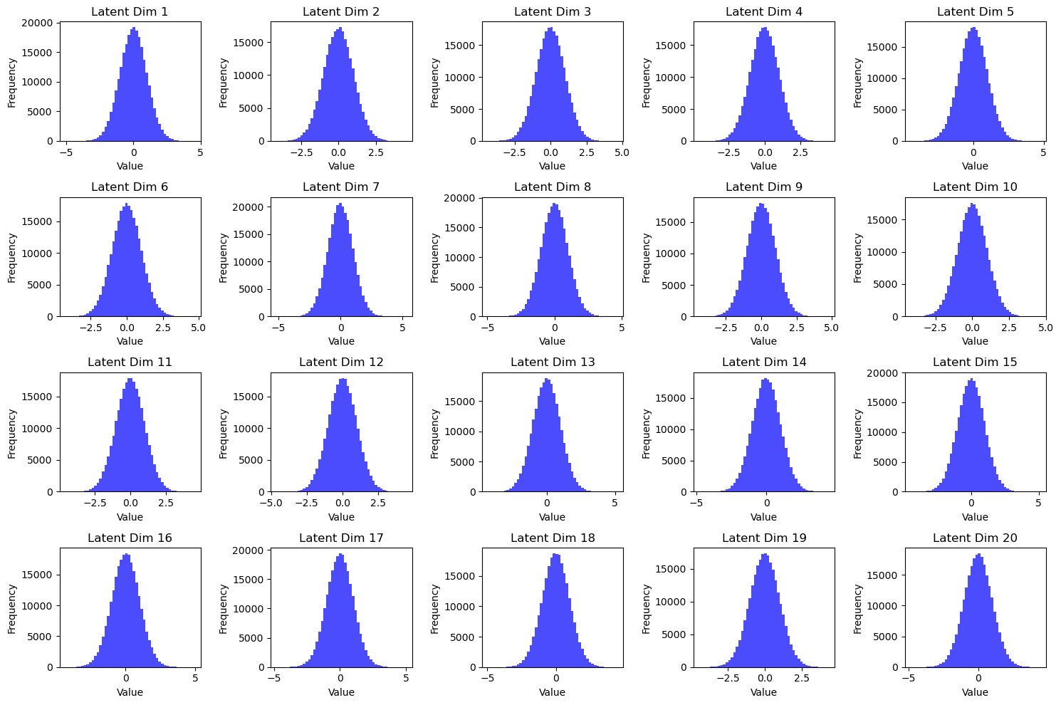
This is not the case for the VAE.

Fig 4: Latent Histograms of VAE

Initializing Geodesic path

We can build a cheap geodesic approximation by computing a knn graph and running Dijkstra. This might prove to be a useful init for the geodesic relaxation. See

Fig 4: Trajectory reconstructed by Dijkstra. The cost of an edge increases exponentially with the euclidean distance. Colors are based on Experiment Time.