Exploring Skip Connections in MLPs

Abstract

This blog post investigates the behaviour of an MLP, where every layer has a skip connection to the last hidden layer. We will see, that such networks tend to perform all relevant computations in early layers, while latter layers tend to learn the identity. One might say that the network learns the most efficient depth. I hypothesize that this is related to the optimal network architecture for a given dataset, but also refute this hypothesis. Further investigation is still needed.

Motivation

Skip connections have proven to be one of the most important concepts in deep learning, as they allow for easy gradient flow during training. One has to distinguish between two different kind of skip connections. The first kind, often called V1 skips before the final non linearity of the residual block. Mathematically speacing we have

\[x' = \sigma (F(x) + Wx ),\]

where x is the input of the residual block, $\sigma()$, the chosen non linearity and $F(x)$ the processing of the block. The processing can range from a simple linear transformation up to a multi head attention block. The linear transformation $W$ may be needed to ensure equal dimensionality. We denote the output of the residual block by $x’$.

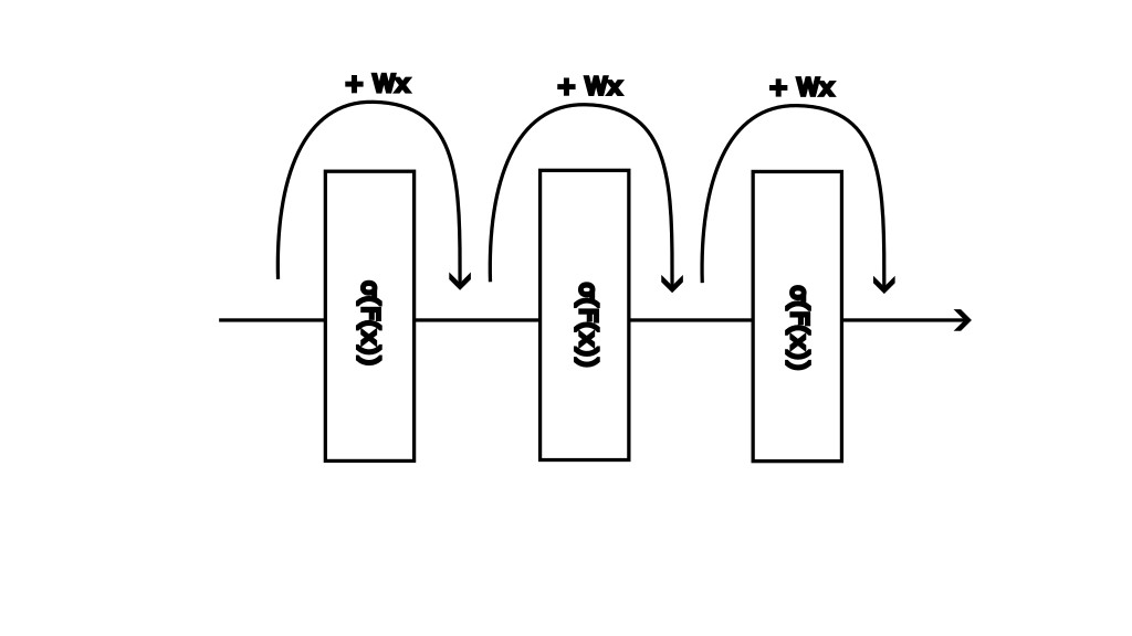
The second kind of residual block, often called V2, performs the skip after the final non linearity of the residual block. The expression thus becomes

\[x' = \sigma (F(x)) + Wx .\]

An illustration of such a skip connection is given by

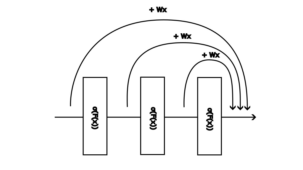
We now modify the structure of V2 blocks. Instead of integrating separate blocks into an MLP, we throw everything together into a sort of telescope structure and allow each layer to skip to the last hidden layer. The following illustrates this approach

Implementation

We simplify the structure by maintaining uniform width across all hidden layers. We can thus use the identity for the skip. The forward pass is defined as follows

def forward(self, x, layers_disabled=None):
    # Initialize array that disables skips during inference, default is [None] * depth
    # i.e. no skip connections are disabled
    if layers_disabled is None:
        layers_disabled = [False]*self.depth
    
    # Zipping layers and layers_disabled array
    layers_out = []
    for idx, (layer, disabled) in enumerate(zip(self.layers, layers_disabled)):
    
        # Feed forward through layers
        x = layer(x)
        
        # If skip_connections is enabled and the layer is not disabled, save the value
        if self.skip_connections and not disabled:
            layers_out.append(x)
    
    # If skip_connections is enabled, add the sum of layers_out to x
    if self.skip_connections:
        x = x + sum(layers_out)
    
    # output layer
    y = self.output_layer(x)
    
    return y 

I save the layer outputs in line 16. The actual skip happens in line 20. The class is written in such a way that I can disable skips during inference, but not during training. This is done via the (misslabled) “layers_disabled” array that is checked in line 15. In addition I can also initialise a network without any skips by setting “self.skip_connections” to False. This results in a usual MLP. What I can not do is to only train with selective skips.

Analysis

This implementation allowes me to analyse the effect of the skip connections on the networks performance. I quickly noted, that disabling skip connections in the latter half has little effect on the accuracy, whilst disabling skip connections in the front half lead to the network realizing a constant function almost immediately. Figure 1 shows then effect. In other words: I can skip the later layers without issues, but if I don’t allow the first layers to skip to the end, everything breaks.

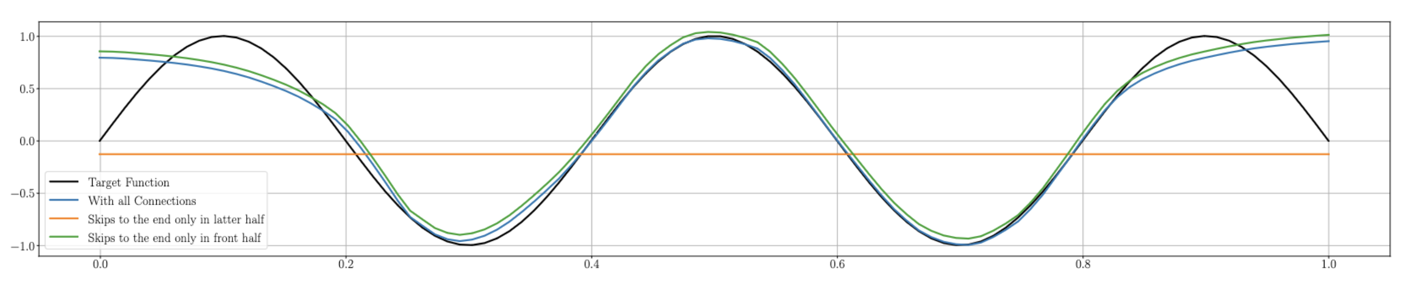Figure 1: A modified ResNet of depth 50, width 64 with ReLU activation. The network was trained with all skip connections enabled. The blue line shows the realized function with all skip connections, the green line shows the realized function if only the first 25 skips are used, the orange line shows the realized function if only the last 25 skips are used.

The irrelevance of the latter skip connections indicates to me, that the network learns to express a constant zero function in the tail end. If this is the case, then it doesn’t matter if we allow a skip in the tail or not, as $0 + 0 = 0$. If this scenario is the accurate, it would also mean, that early skips are highly relevant, as if they are suppressed, then the network would have to push everything through these constant zero functions, immediately zeroing out the resulting function. Such behaviour would support the behaviour seen.

Investigating Layer Activity

To support this hypothesis I looked at the average magnitude of the weights of different layers, the idea being, that if it is close to zero, that the layer essentially realizes the zero function and I conjuction with an earlier skip essentially the identity. I ran a simple average over each weight matrix and plotted them by layer. This is shown in figure 2.

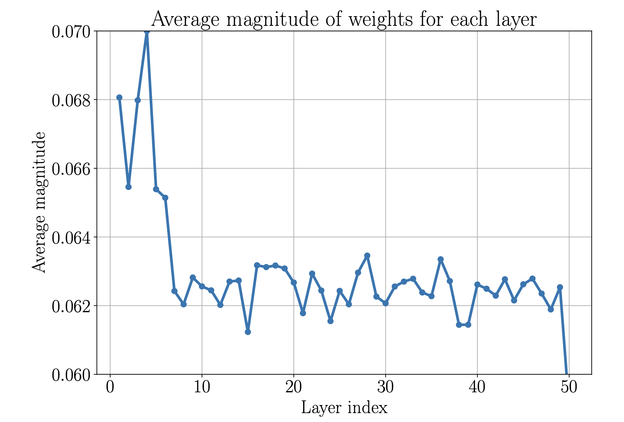Figure 2: Average magnitude of the weights the hidden layers of the modified V2 model. We can see, that the most significant processing happens in the first five to seven layers. Layer 50 is usually an outlier, as it receives all the skip connections including one from itself.

Just as a sanity check we compare this to a normal V2 model and get the layer activity seen in figure 3.

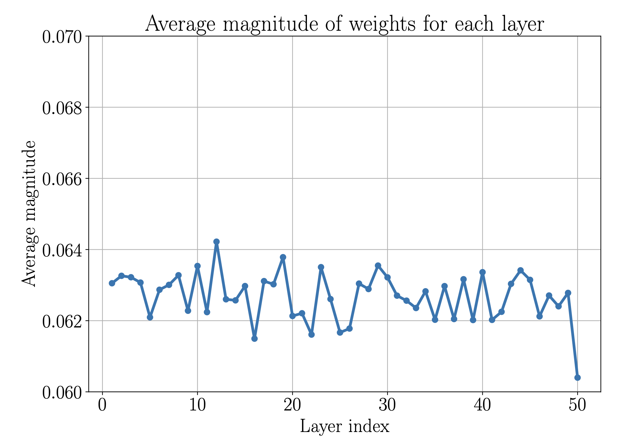Figure 3: Average magnitude of the hidden layers of a ResNet V2. Here the processing seems to be equally distributed among the layers.

Both networks are of depth 50 and width 64, use ReLU activations and were trained on the same data set for 2000 epochs using Adam.

Investigating Self Truncation

My idea now was, that the skip connections essentially allow the network to always truncate itself. Every layer in essence acts as the final hidden layer, which could mean that they compete in some way. Thus if the first five to seven layers out compete the others, they may have some inherent advantage. This may extend to normal MLPs as well, in the sense that if I make my network too deep, I might not be able to utilize that advantage, as the later layers will make the training of the first layers harder.

I did some more analysis by disabling selective layers, which again showed the importance of the first seven layers and thus formulated my loose hypothesis: “The activity of the first layers reflects their learning efficiency compared to later layers”. Finally I wanted to see if this could also be seen in normal MLPs. To test this I initialized MLPs with the same width of 64, ReLU activations with depth ranging from 2 to 50 and trained these networks using the same training routine as before on the same training data in 100 epochs. To quantify the error I employed a Monte-Carlo method by generating 1000 random points $x_i \in \operatorname{supp}(\text{Training Data})$ and calculating

\[\text{error approximation} = \frac{1}{1000}\sum_{i=1}^{1000} \left( \sin(x_i) - \Phi_\text{depth}(x_i) \right)^2,\]

where $\Phi_\text{depth}$ is the inference of an MLP with specified depth. The results are shown in figure 4.

Figure 4: Monte-Carlo error approximation for ReLU MLPs of different depth. Each network was given the same training dataset and trained in the same number of epochs. One can clearly see, how networks between depth 8-13 seem to have an advantage in this rather short training routine.

This does not quite support my Hypothesis, as the gains start after the first seven layers. Maybe the hight activity indicates, that the layers are actually needed or maybe it is just an insignificant anomaly of the modified ResNet. Testing this hypothesis on different network sizes with different tasks is needed to be more confident in the hypothesis.

I want to make two remarks on figure 4:

• One can nicely see the depth at which the network gets too deep to be trained without skip connections
• The plot is highly dependant upon the training amount. If we increase the epochs we can make shallow networks with comparable accuracy to medium sized networks.

Further Ideas

The first weight update should be highly dependant on the chosen weight initialization scheme. Let’s assume for a second, that the network is initialized with zero bias and the identity for the weights. In this case each layer gets exactly the input data and directly escapes to the last layer. Therefore they are all identical and should receive exactly the same gradient. This changes in every subsequent weight update, as layers no longer realize the identity. The question is now, if the early layers now carry a larger gradient. This seems a bit counter intuitive, as any change made to early layers should also effect the last layer through every subsequent skip. Latter layers in contrast have ever less skips to influence this layer and should thus receive larger gradients to make up for this reduced effect strength. It might be interesting to initialize the network as described above and to investigate the gradient behaviour.

Now lets assume He initialization for the network. In this case each layer immediately receives a different input and therefore the first gradient should be unique for each layer. In other words: We immediately are in this chaotic behaviour. The question is now if the first weight update is of high importance. These considerations however still do not explain why we see the drop of in weight magnitude throughout the layers. It might also be interesting to build a very small network and investigate each weight update individually to better understand the drift of the latter layers to the zero function.

As far as I’m aware PyTorch initializes ReLU networks using He initialization. Therefore the answer to this drift should not be found in the first gradient update. I leave the investigation here for now and might return to it later.