When Massive Parallelism Is Not Enough: Optimizing the Hamming Matrix

Topological Data Analysis (TDA) is concerned with finding topological invariants of a data set. This allows us to find circular relationships in datasets, as a circle can be seen as a hole in the data manifold and hence can be described by topology. This can for example be used to find beneficial mutations in viral evolution (see for example [Bleher et al.]).

To perform the TDA, we are given a point cloud dataset $X \subset \mathbb{R}^d$ with a metric $d(x,y)$, where $x, y \in X$. We now calculate the distance between each data point and summarize it in a distance matrix. We then generate the Vietoris–Rips complex from this Hamming matrix and compute the persistent homology of the dataset, which summarizes the topological invariants.

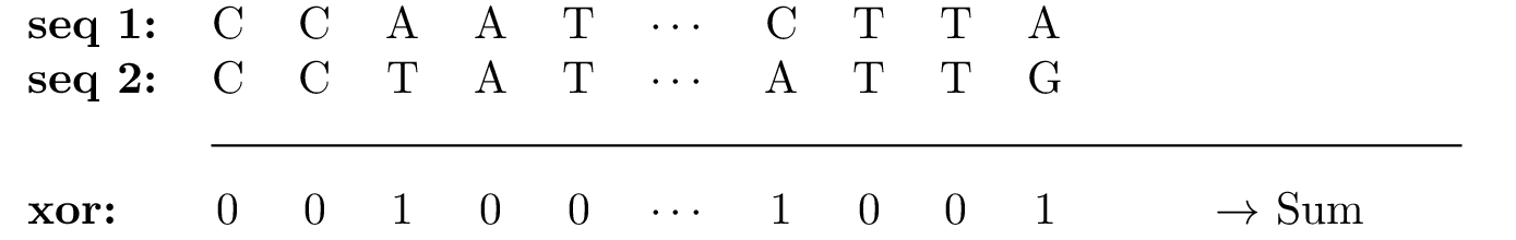
We can apply this approach to a collection of viral genomes. The natural metric here is the Hamming distance, which counts the number of positions where two genomes differ. Thus to compute an entry in the Hamming matrix we load in two sequences and compare them at each index with a simple XOR. Afterwards we sum along the XOR sequence to get the distance between the two sequences.

Notice how each comparison is independent of all the others and that computing an entry in the Hamming matrix is independent of all other entries. My initial naive thought was that using the right tensor operations in PyTorch, we could perform all these computations simultaneously and then simply sum up the results. This seemed like exactly what GPUs are built for. Boy was I wrong!

The naive Approach

The dataset can be viewed as a $n \times d$ matrix where $n$ refers to the number of genomes. We can create $n$ shallow copies of each sequence along a new index leading to the following tensor: 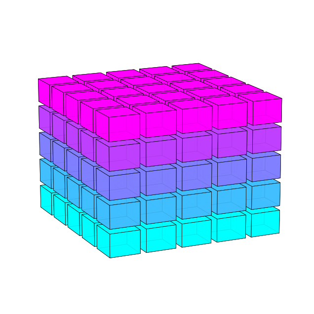Here the sequences go from front to back. Each unique sequence is given a unique color, every copy is assigned the same color. The new index goes from left to right, hence leading to horizontal stacking of the replicated data matrix.

We can now transpose this tensor and overlap it with itself to get the interaction of each sequence in the dataset with all the others. Afterwards we perform the XOR at every overlapping sequence creating a new 3D tensor. We now sum front to back to get the final Hamming matrix. This can be summarized in the following animation.

The beauty of this approach is twofold: First all comparisons happen in principle at the same time thus maximizing parallelization and second it is very easy to implement in PyTorch:

n, d = tensor_dna.size()
left = tensor_dna.unsqueeze(1).expand(n, n, d)
top = tensor_dna.unsqueeze(0)
diff = left != top
hamming_matrix = diff.sum(dim=2)

Whilst this makes for some very elegant code, it fails spectacularly in comparison to even the simplest CPU implementation. It took me a lecture on GPUs to find out why.

The very Basics of GPU computing

A modern Nvidia GPU basically consists of

• Streaming Multiprocessors (SMs): Computing blocks with local memory that can process data from and into local memory and request new data from global memory
• Global Memory: A global memory resource, that can be accessed by all SMs
• A lot of infrastructure connecting everything

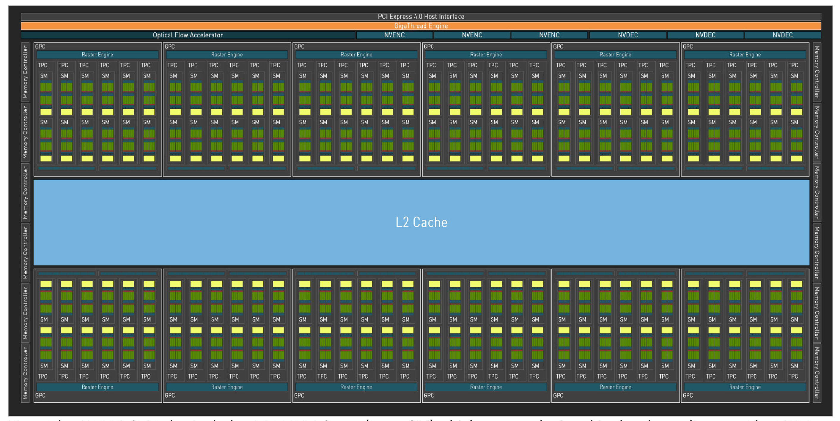An overview of the architecture of an RTX 4090. Notice the abundance of SMs on the chip. Each SM has its own memory and L1 cache. The L2 cache is shared amongst all SMs on the die. Global memory is an off-chip resource and thus not shown. Also, the RTX 4090 is a gaming GPU and thus has a lot of functionality for computer graphics. It can be safely ignored for this discussion. (Source: Ada Lovelace Whitepaper)

Instead of executing functions on a GPU, CUDA instead launches a kernel. It is in many ways similar to a C++ function, but instead of executing one, it spawns many different threads executing the same function. To control this parallelism, we specify a block and a grid size.

The block size determines how many threads of the function we want to spawn on a single SM. Different threads execute the same instructions on different data. We can execute up to 1024 threads on a single SM. For the actual execution the GPU groups up to 32 threads into what is called a warp. A scheduler now chooses a warp for execution, which is then executed in a SIMD style. Thus we pretty much always execute 32 threads at the same time on a single SM. As all threads in a block reside on the same SM, they can communicate with each other. We need to keep in mind however that a priori it is not guaranteed, that all threads are at the same instruction of the kernel. To prevent threads from illegal memory accesses or working on stale data we need to synchronize them. For more on this see BSP.

If 1024 threads are not sufficient, we can use the grid size parameter. It determines on how many SMs the function will be executed. Consider for example a grid size of 20 with a block size of 512. The GPU will now execute the function on 20 SMs, each with 512 threads. The drawback here is that threads can not communicate or even be synchronized across different SMs. Thus, the only way for a thread on SM A to pass information to a thread on SM B is to write the result to global memory, terminate the kernel, and then relaunch it. This kernel relaunch is the only way to guarantee that all threads from a kernel are at the same instruction of the kernel.

One of the key tricks that GPUs use to achieve high performance is called parallel slackness. Unlike CPUs, GPUs can switch between different warps extremely quickly when a warp stalls, such as when waiting for data from global memory—a delay that can easily cost 100 clock cycles. Instead of idling during this wait, the GPU scheduler immediately switches execution to another warp that’s ready to run. This rapid context switching effectively hides memory latency and keeps GPU resources utilized. However, to fully benefit from parallel slackness, the GPU needs enough warps queued up and ready; otherwise, the SM stalls and performance suffers. GPUs use a similar strategy at the block level, but that’s beyond our scope here.

Parallel slackness in action: The SM works on a warp until it stalls. It then switches to a warp that is ready for execution. Stalled warps should become ready for execution as soon as the high latency operation, such as a memory access, is completed. If no warp is ready for execution, the entire SM stalls.

The Culprit of the Hamming Matrix: Arithmetic intensity

Arithmetic intensity measures how many operations are performed per byte loaded. We usually target a value of at least 100. This ensures that by the time new data needs to be loaded in, another warp has already completed its memory request. Our Hamming distance is in many ways the worst case. We can represent each base pair as a single byte. Per base pair we only need to perform a single XOR operation and a few additions, which are highly optimized on GPUs. Thus we are constantly stalling as we’re waiting for the next base pairs to be loaded in. I suspect that this is where the PyTorch implementation is failing.

Fortunately, CUDA allows us to parallelize not only execution but also memory transactions by bundling multiple data fetches into fewer memory operations. From a machine learning perspective we might say that we work in batches. This however takes an explicit effort on the part of the programmer. I found the most important optimization to be transposing one of the arrays on the CPU before copying both onto the GPU. This allows the memory controller to load in the data in a coalesced manner, if we carefully reason through what data needs to be loaded when. What is meant exactly by this is again beyond the scope of this post, but a good reference can be found in [Kirk et al.].

Nsight Compute, a profiler by Nvidia gives us some insight about the performance of our code. The most important for us is the estimate of the computational intensity. In contrast to the arithmetic intensity, which is concerned with the theoretical arithmetic, the computational intensity is concerned with the operations per byte of the actual performance. To understand our kernel Nsight Compute provides the roofline chart.

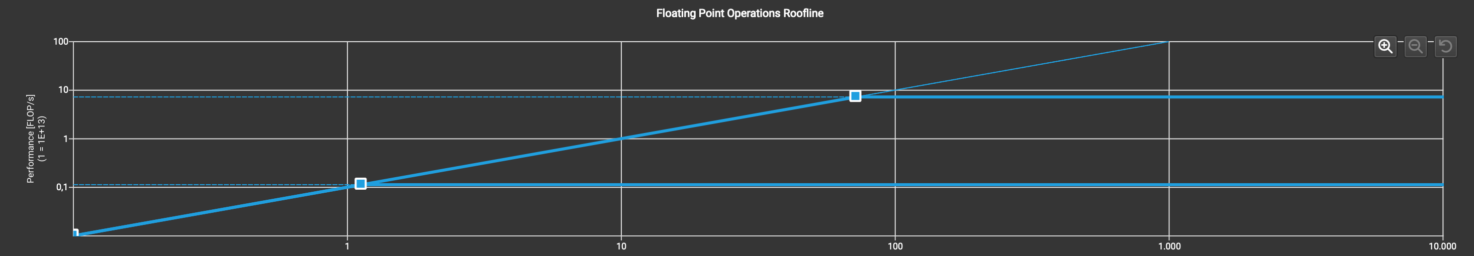The roofline chart plots computational intensity against peak performance. There are two break-even points, one for fp32 and one for fp64. If we’re left of these break even points our kernel is memory bound. The maximum performance is then given by the solid blue line. Any improvements in computational speed are negated by warps stalling as they wait for new data. Kernels sitting to the right of the break-even point are referred to as compute bound. Here smarter computations do bring tangible performance benefits.

For the longest time I though that Nsight Compute was not properly profiling my kernel, as I did not find the marker indicating our performance in the roofline plot. It is however there, at the bottom left corner. Notice how it is actually below one as we’re performing some clever byte packing (and also unfortunately load in some redundant data).

Nevertheless, with careful memory management, GPUs can still significantly outperform CPUs in computing Hamming distances. I currently benchmark a 20 fold improvement against a SIMD based C++ implementation. We do however lose again to the CPU when it comes to very large data sets that no longer fit onto the global memory of the device. Here we’d have to stream in data from system memory over PCI express, which carries a much higher penalty than the already very high penalty of global memory accesses.

Final Verdict and a Note on Future Developments

As we have seen, for good GPU performance we not only need to construct problems that can be broken down into independent sub problems, we also need a sufficiently high arithmetic intensity to not stall for memory requests. Fortunately, matrix multiplication—the backbone of modern machine learning—requires $2N^2$ loads and $2N^3$ operations when multiplying two square matrices. Thus our arithmetic intensity scales linearly in matrix size.

As stated I currently target an arithmetic intensity of at least 100. With future GPUs we do however expect both the compute as well as the memory sub system to improve. We can quickly estimate a good target for any GPU by dividing the peak Float32 performance by the Memory bandwidth. While simplified, this helps guide initial performance expectations and optimization efforts. For the 4090 this gives a target of ~80. Generally we however expect that compute improves faster than memory. Thus in the long run kernels need to be more compute heavy to fully utilize a GPU. Thus, neural networks will likely need to grow even larger to scale effectively with future increases in computational capability.

References

[Bleher et al.] Bleher, Michael et al. “Topology identifies emerging adaptive mutations in SARS-CoV-2” arXiv preprint arXiv:2106.07292 (2021)

[Kirk et al. ] Kirk, David and Hwu, Wen-mei “Programming Massively Parallel Processors: A Hands-on Approach”