The Genodesic

In Biology we’re often confronted with static snapshots of dynamic systems. A key task is to reconstruct the underlying dynamics from this snapshot. A prime example of such a task is trajectory reconstruction, where we try to find the typical path a cell takes whilst undergoing some process.

If we now assume that the system we’re observing is ergodic, then a sufficiently large sample size will contain all intermediate stages of the process. Hence the trajectory reconstruction becomes essentially a regression task on the dataset.

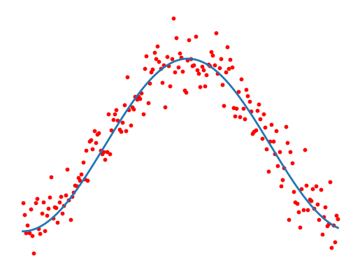
Fig 1: We measure multiple cells, which all undergo the same dynamical process. Finding the typical development path boils down to computing a regression.

Finding such a regression path seems easy at first glance. But in the high dimensional data spaces commonly found in bioinformatics, the curse of dimensionality may quickly strike. Specifically the Euclidean metric can break down with an increase in dimensionality (see [Beyer et al.]). This is the detriment of most regression algorithms, such as principle curves, who often minimize some kind of Euclidean metric to the data. In the following we will not necessarily try to replace the Euclidean distances. Instead we want to enhance it with additional information to make it more robust in higher dimensions.

This blog post is concerned with the big picture concept of my master’s thesis and will delve a bit into how I simplified the modeling paradigm of an Information Geometry based regression algorithm, as well as into some technical aspects around the smoothness and stability of score estimates in the Hyvärinen sense. We will apply these techniques to single cell sequencing count data of cells undergoing stem cell reprogramming.

Mixing in some Information Geometry

[Sorrenson et al.] introduces the idea of constructing Geodesics with respect to a Fermat metric. In less mathematical terms this means the following: In Riemannian Geometry we allow our metric to vary as a function of the current position. One such choice for a metric is given by the Fermat metric, which rescales the normal Euclidean metric according to some property. In our case we rescale the Euclidean metric with respect to the density of the dataset at that point in such a way, that distances in high density regions become shorter, whilst distances in low density regions are enlarged. As our metric is derived from data, we’re firmly in the Information Geometry world. Our metric is given by

\[g(u,v) := \frac{\langle u,v \rangle}{p^\beta},\]

where $\langle u,v \rangle$ is the usual Euclidean metric, $p$ the density at the current position and $\beta$ some hyperparameter.

A Geodesic is now a curve, that (under appropriate assumptions) minimizes the length traveled between two points. In our case this means, that a curve going through the data will be shorter than a curve taking shortcuts through low density regions, as the distances are shorter where the data is. This has the effect, that solving a goedesic with respect to a Fermat metric will generate a curve, that will try to stick to the data.

In more mathematical terms, a geodesic $\gamma:[0,1] \to M$ minimizes the Length functional

\[L(\gamma) := \int_0^1 \sqrt{g_{\gamma(t)}(\dot{\gamma}(t),\dot{\gamma}(t))} dt,\]

where $g$ is the Fermat metric as defined above and $u$ and $v$ are tangent vectors at $\gamma(t)$. For length minimization we need to ensure that we use the correct Levi-Civita connection for our Geodesic equation $\nabla_\dot{\gamma} \dot{\gamma} = 0$. At the end we need to solve the following PDE (more details in [Sorrenson et al.])

\[\ddot{\gamma} - 2\beta (s(\gamma) \cdot \dot{\gamma}) \dot{\gamma} + \beta s(\gamma) ||\dot{\gamma}||^2 = 0,\]

where $s = \frac{\partial \log p}{\partial x}$ is the score in the sense of Hyvärinen and $\vert\vert \cdot \vert\vert$ the Euclidean norm. This PDE may be solved via a relaxation scheme, where we need to provide the start and endpoint we want to connect geodesically. We may also reframe it into an IVP, allowing us to predict the movement of a cell without a known endpoint. In this case however we also need to provide an initial direction of movement. Critically though in both cases we need access to the score of a position in the dataspace. We will return to this in just a second.

Fig 2: Our relaxation of the Geodesic equation in action. We start with some initial path proposal connecting our desired start and end point. We update the curve using the score of the dataset.

About the Initialization

If we want to solve the PDE via relaxation, we need to provide it with an initial solution that will be iteratively refined. An initial guess might be given by the straight line connecting the start and end point. This proposal however is usually so far off the actual solution, that the relaxation scheme will fail to converge. Hence we need to come up with a smarter initial guess. [Sorrenson et al.] suggests to find an initial proposal using graph based methods. Specifically we construct a k-nearest neighbour (knn) graph with respect to the Euclidean norm. We then update the weights of the edges in the graph based on the density between the two nodes of the edge. A path proposal is now given by Dijkstra, which finds the shortest path between two points in the density based graph. The idea for the update of the edge weights is that locally the geodesic between two datapoints is given by a straight line in the Euclidean sense. The edge weight is approximated using

\[dist(x_1, x_2) = \sum_{i = 1}^s \frac{|| y_i - y_{i-1}||}{p\big( y_{i - \frac{1}{2}} \big)},\]

where $y_i$ are linear interpolates such that $y_0= x_1$ and $y_s = x_2$. Notice how we need to directly estimate the density of a point here instead of just the score.

The Problem with the Scores

[Sorrenson et al.] proposes to estimate the data via some normalizing flow (RQ-NSF [Durkan et al.]). This yields density estimates and in principle also the score via Autodiff. They noticed however, that calculating the score this way tends to produce rather noisy estimates. Hence, they resort to learning the score separately via sliced score matching to get around the AD stability issues. This separates our likelihood modeling from our score modeling. I wanted to investigate whether we can get around this issue by deriving the likelihood from a score model, rather than deriving the score estimate from a likelihood model.

The relevant comparisons are not quite straight forward. I’ve tested many different classical normalizing flow frameworks and whilst RQ-NSF is the most successful approach, it still is not convincing (see figure 7). Only when moving to a continuous normalizing flow framework do the results become acceptable. A relevant point of comparison is CellFlow by [Palma et al.], where they model sequencing count data using OT-CFM [Tong et al.]. This model can generate likelihoods by accounting for the divergence of the NeuralODE, as well as score estimates by employing an adjoint solver. It is thus a successful model, where the score is derived from the likelihood.

For my approach I choose to employ the VP-SDE from [Song et al.]. Unsurprisingly the generative capabilities of this approach are generally better then OT-CFM or RQ-NSF (see figure 7). We can also sample the network at $t=0$ to get a score estimate of the distribution. This is both in theory and in practice equivalent to DSM. Furthermore by considering the associated probability flow ODE ([Song et al.] appendix D), a VP-SDE set up can also provide likelihood estimates. Notice how the set up is mirrored in comparison to the original approach [Sorrenson et al.]. We directly model the score and derive a likelihood estimate from it. Thus we expect the scores to be somewhat better behaved. Another important side effect of this approach is, that generating a score via Autodiff, especially through an adjoint solver as found in the OT-CFM approach, is computationally speaking much more expensive than a simple neural net evaluation found in the VP-SDE approach.

We compare the score estimate on two benchmarks. By Taylor’s theorem we expect for a sufficiently regular function

\[s(x + \epsilon) - s(x) = s'(x)\epsilon + o(\epsilon^2),\]

where $s’$ is the Jacobian of the score estimate. The key insight here is, that a stable score estimate should behave linearly under small perturbations until running into numerical issues. We hence compare $\vert\vert s(x + \epsilon) - s(x)\vert\vert $, where $\epsilon$ is just a deterministic perturbation vector. The results are shown in figure 3.

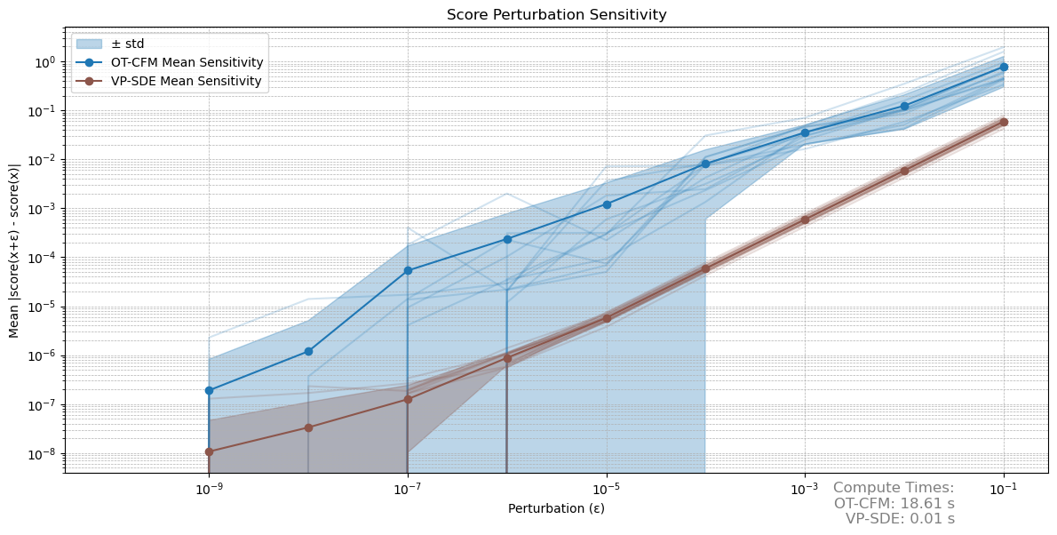Fig 3: Comparison of the stability of the score estimates under small perturbations. We perturb the score at 12 random datapoints. The average is plotted in high opacity.

Notice how the VP-SDE approach both demonstrates a more linear behaviour, but also a lower variance between samples. For the OT-CFM approach the variance is at times so high, that it drops out of our logarithmic plot. Eventually both approaches run into numerical issues, but I’d argue that the VP-SDE approach is generally more stable and well behaved.

Another important property a good score estimate should have is a consistent direction under small perturbations. If the perturbation is small enough, then again by Taylor we have

\[\begin{align*} s(x)^\intercal s(x + \epsilon) &= s(x)^\intercal (s(x) + s'(x) \epsilon + o(\epsilon^2)) \\ &= s(x)^\intercal s(x) + s(x)^\intercal s'(x) \epsilon + o(\epsilon^2), \end{align*}\]

in words again a linear relationship. We again evaluate both models over multiple runs. The results are shown in figure 4.

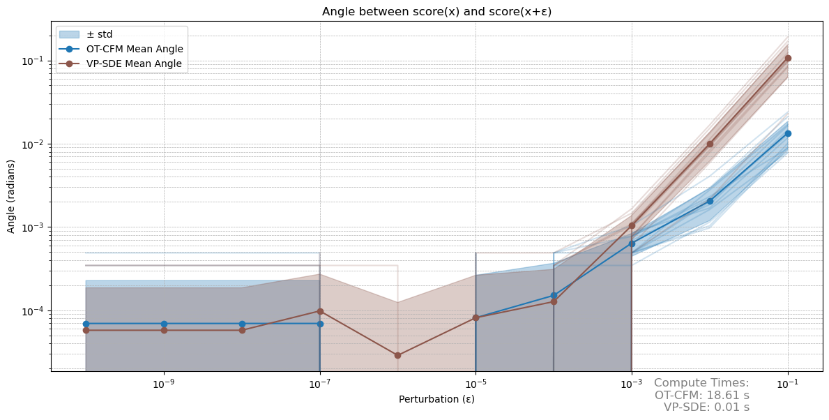Figure 4: Evaluating cosine similarities over perturbations. Again the variance may drop out of the log plot.

In this metric both approaches perform similarly. Interestingly enough we run into numerical instability faster then in the other benchmark. In our downstream application of the score estimate the VP-SDE approach also outperforms the OT-CFM approach, whilst requiring much less compute. These results aren’t necessarily surprising, as the adjoint solver used in the for the OT-CFM approach needs to not only solve an ODE, increasing compute, but also account for the divergence along the flow. Estimating this divergence with the Hutchinson trace estimator introduces Monte-Carlo effects. Thus the VP-SDE approach is generally to be preferred, as it not only provides smooth score estimates, increasing the stability of the geodesic relaxation, but also unifies score and likelihood modeling into a single framework.

A quick Demonstration of the Genodesic

Going back to our application at hand we can solve the geodesic equation between two datapoints in the dataset. We use the VP-SDE model to both find the initial path proposal, as well as solving the geodesic equation via relaxation. This allows to perform a regression which is a bit more stable in higher dimensions, as we’re not relying as much on euclidean distances. An example of such a regression is shown in figure 5.

Fig 5: A regression in the Schiebinger Dataset. The initial proposal is in red, the relaxed curve in green. The coloring of the cells reflects the wallclock time provided by the dataset. The plot is a 3D UMAP of the 16 dimensional latent space. All computations are done in the latent space.

Evaluating Pseudotimes

The reason why we benchmark on the Schiebinger Dataset is, that this dataset provides a wallclock time. Our Genodesic is also able to generate a pseudotime, as it is a parameterized curve. Even though the two times are not on the same scale, we can still compare their ordinality. We do this by considering the 10 nearest neighbours in the dataset of some points in our curve and averaging over them. This allows us to find the wallclock time in the immediate vicinity of the curve. We compare this estimate to our curve parameter. A good pseudotime estimate should be always rising in the wallclock time. If our wallclocktime decreases along our pseudotime, this would mean that our curve would go back in time and thus not capture the dynamics correctly.

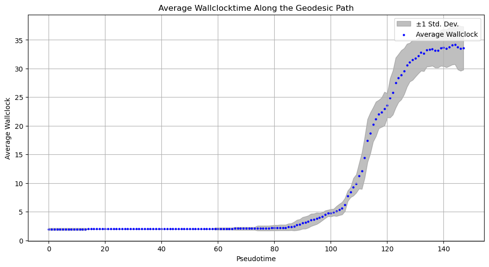
Fig 6: Comparing the pseudotime to the wallclock time. A perfect estimate would be a diagonal line. Whilst the results aren’t great, they’re at least not terrible 🤷. The ordinality seems to be largely correct.

Generative Modeling as a Side Effect

All our approaches can not only provide density and score estimates, but can also perform generative modeling. We can use this as a sort of benchmark to get an impression about whether the model is actually capable of learning the underlying data. To benchmark this capability, we’re going to let all models generate exactly as many datapoints as there are in our training dataset. For each real datapoint we can then calculate the 10 nearest neighbours in both the real as well as the generated dataset. Dividing by 10 gives us a fraction for each datapoint, that indicates what the share of artificial datapoints around any real datapoint is. For a good model we’d expect this fraction to sit around 0.5, indicating an equal share of real and fake data. This provides a spatially-resolved view of model fit, unlike a single validation loss value, revealing which parts of the data manifold are well-captured or missed. We can also invert this analysis and consider the share of fake datapoints around each fake datapoint, indicating regions in the generated data, where the model invents stuff that is not backed by the data. The results of this analysis are shown in figure 7.

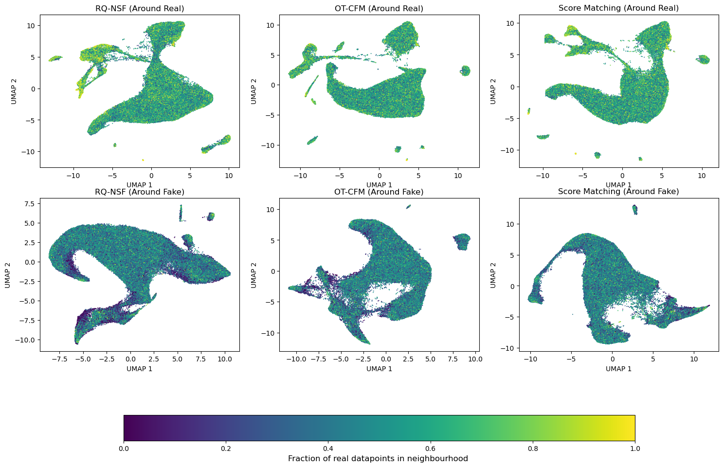Fig 7: Comparing generative capabilities. The top row shows the fraction of real datapoints around real datapoints. It thus answers “What did the model miss”. The bottom row shows the fraction of real datapoints around fake datapoints. It thus answers “What did the model invent”.

We can see in the top row of figure 7, that RQ-NSF is not capable of capturing the entire data manifold. There are significant regions, where there are essentially no datapoints around real datapoints. In contrast both OT-CFM as well as the VP-SDE seem to be largely alright on that front. In the bottom row we can see that both RQ-NSF as well as OT-CFM have parts, where there are only few real points around some generated points. Here the models are generating points in regions, that are not covered by the actual data. They are thus inventing data. Whilst these regions are also present in the VP-SDE model, I’d argue they’re less pronounced. This is actually really important for our genodesic, as a model that “fills in the blanks” will lead to a trajectory going through “invented biology”. Hence I conclude, that also on this front my VP-SDE approach outperforms the other models, as it not only beats the other models on all investigated benchmarks, but also makes the key improvement of combining the likelihood and score modeling needed into one unified model.

Minor Remarks

Apart from the usual Bioinformatics workflow of filtering count datasets to find highly variant genes, we are also using an Autoencoder to reduce ~1500 highly variable genes to a 12 dimensional latent space. This Autoencoder replaces the standard PCA. Instead of a standard reconstruction loss however, it is better to explicitly consider the Negative Binomial (NB) distribution of count data. Whilst this methodology is a bit novel, I still didn’t find it appropriate to include it in the discussion above, as geodesic trajectory reconstruction works in general continuous dataspaces. Yet still, the NB-Autoencoder should merit a future blog entry.

Possible Improvements

Currently most compute is spend on generating the initial path proposal. This is because we calculate a knn of the dataset and then update each edge using the density estimated provided by the probability flow ode. Thus we have to run a lot of network evaluations per edge for a lot of edges. We do this as a naive proposal such as a straight line usually goes through very sparse regions of the latent space. The scores in these regions are very uninformative, leading to a failure of convergence. Notice how this is one of the problems also encountered and solved in [Song et al.]. Here they noticed, that we can get more sensible score estimates for sparse regions by inflating the noise perturbation. As this is already the model we employ, we might construct a relaxation scheme, where we initialize with a straight line and gradually reduce the noise over time. Thus our early curve will still have informative scores, whilst later relaxation steps should be able to make use of more detailed score estimates. Thus we may be able to completely cut out the graph based parts of our pipeline, significantly reducing compute.

References

[Beyer et al.] Kevin Beyer, Jonathan Goldstein, Raghu Ramakrishnan, Uri Shaft “When Is “Nearest Neighbor” Meaningful?”

[Sorrenson et al.] Peter Sorrenson, Daniel Behrend-Uriarte, Christoph Schnörr, Ullrich Köthe “Learning Distances from Data with Normalizing Flows and Score Matching”

[Palma et al.] Alessandro Palma, Till Richter, Hanyi Zhang, Andrea Dittadi, Fabian J Theis “cellFlow: a generative flow-based model for single-cell count data”

[Song et al.] Yang Song, Jascha Sohl-Dickstein, Diederik P. Kingma, Abhishek Kumar, Stefano Ermon, Ben Poole “Score-Based Generative Modeling through Stochastic Differential Equations”

[Tong et al.] Alexander Tong, Kilian Fatras, Nikolay Malkin, Guillaume Huguet, Yanlei Zhang, Jarrid Rector-Brooks, Guy Wolf, Yoshua Bengio “Improving and generalizing flow-based generative models with minibatch optimal transport”

[Durkan et al.] Conor Durkan, Artur Bekasov, Iain Murray, George Papamakarios “Neural Spline Flows”